Part two of the modelling pair, after every ML model and when to use it. That one covered tables and images. This one is language, and it’s all architecture: no training recipes, no prompting, no RAG. Just what the models are and why they ended up shaped this way.
Here’s the thing about NLP: it has been solving the same problem for sixty years. Text is symbols, maths needs numbers, and every era of NLP is just a different answer to how do you turn one into the other.
What makes the story worth knowing is that each answer broke in a specific way, and the next thing was built to fix exactly that break. Learn it as a chain and you never have to memorize it.
1. What Anybody Was Actually Trying to Do
None of this was invented for its own sake. Four jobs drove the whole field, and knowing which one drove which invention is most of the story:
| The job | What it means | What it drove |
|---|---|---|
| Find the right document | someone types a query, you rank a million documents | TF-IDF, and every embedding model since |
| Guess the next word | which word plausibly comes next | n-grams, then RNNs, then every LLM alive |
| Turn one sequence into another | English in, French out | seq2seq, attention, the transformer itself |
| Label the text | spam or not, which words are names, is this angry | classification heads, BERT-style encoders |
Say it like this: NLP has four jobs, and almost every architecture in this post was invented for one of them and then turned out to be good at the others.
That last clause matters. TF-IDF was built to rank search results and ended up as the default text classifier baseline. The transformer was built to translate faster and ended up running everything. The pattern repeats so often it’s worth expecting.
2. The Whole Post in One Table
| Idea | What it fixed | What it broke |
|---|---|---|
| One-hot | text becomes numbers at all | no meaning, vector as long as the vocabulary |
| Bag of words | document as one vector | word order gone entirely |
| n-grams | a little local order | vocabulary explodes |
| TF-IDF | weights what’s actually informative | still zero semantics |
| word2vec / GloVe | real meaning, dense, small | one vector per word, whatever the sentence |
| RNN | context, any length | sequential, forgetful, slow |
| LSTM / GRU | the forgetting | still sequential |
| seq2seq | variable in, variable out | everything squeezed through one vector |
| Attention (2014) | that bottleneck | still recurrent underneath |
| Transformer | recurrence, so it parallelizes | cost grows with the square of length, no sense of order |
| Positional encoding | the order problem | doesn’t extrapolate past training length |
| MQA / GQA / sliding window | memory and the quadratic cost | some quality, some recall |
| SSM / Mamba | quadratic cost entirely | exact lookup of anything earlier |
Read that top to bottom and you have the plot. The rest of this post is the detail.
3. Counting Words
3.1 One-hot
Give every word in your vocabulary a slot. A word becomes a vector of all zeros with a single 1 in its slot.
Say it like this: one-hot turns a word into its row number, written the long way.
The problem shows up the moment you try to use it. With a 50,000-word vocabulary, every word is a 50,000-long vector that is 99.998% zeros. Worse, every pair of words is exactly the same distance apart. “cat” and “kitten” are as unrelated as “cat” and “bureaucracy”. There is no meaning in there at all, because you never put any in.
3.2 Bag of Words and n-grams
Built for: guessing the next word. n-gram language models were what made early speech recognition and autocorrect work, by asking which word usually follows these two.
Count how many times each word appears in a document and you get one vector for the whole document. That’s bag of words, and the name is honest: you shook the sentence until the word order fell out.
Say it like this: bag of words knows what you said, not the order you said it in.
“dog bites man” and “man bites dog” are identical. So n-grams keep short runs of words as single units: bigrams treat “not good” as one token, which is the difference between a positive and negative review.
The cost is brutal arithmetic. A 50,000-word vocabulary has 50,000 unigrams, but 2.5 billion possible bigrams and 10\(^{14}\) trigrams. You never see most of them, so the matrix gets enormous and emptier at the same time.
Where you’d still use it: bigrams on top of TF-IDF, for a text classifier you need working this afternoon.
3.3 TF-IDF
Built for: ranking search results. TF-IDF came out of information retrieval in the 1970s, where the question was which of a million documents best matches a query.
Raw counts have an obvious flaw: “the” appears in every document, so it dominates every vector while telling you nothing. TF-IDF fixes that by asking not just “how often is this word here” but “how unusual is it that this word is here at all”.
Say it like this: TF-IDF rewards words that are common in this document and rare everywhere else.
$$\text{tfidf}(t,d)=\underbrace{\text{count of }t\text{ in }d}_{\text{term frequency}}\times\underbrace{\log\frac{N}{\text{docs containing }t}}_{\text{inverse document frequency}}$$That second factor is the whole trick. A word in every document gets \(\log(N/N)=\log 1=0\) and vanishes. A word in 1% of documents gets \(\log 100\) and gets loud.
Pros: fast, sparse, interpretable (you can read which words drove a prediction), and genuinely hard to beat on small labelled text sets. Cons: no semantics whatsoever. To TF-IDF, “excellent” and “superb” are two unrelated columns.
Trap: “TF-IDF is obsolete.” It is not. It’s the baseline you run in twenty minutes before you spend two weeks on a transformer, and it is embarrassingly competitive on narrow domains with a few thousand labelled examples. See the model selection post.
4. Tokenization: How You Chop Text Up
Before anything sees a word, something has to decide what counts as a word. This choice looks boring and explains an alarming number of LLM quirks.
| Scheme | Vocabulary | Sequence length | The problem |
|---|---|---|---|
| Word-level | huge (100k+) | short | unknown words are simply impossible |
| Character-level | tiny (~100) | very long | a character carries almost no meaning |
| Subword | ~32k to 128k | medium | the sensible compromise everyone uses |
Say it like this: subword tokenization keeps common words whole and chops rare ones into pieces, so nothing is ever truly unknown.
BPE (byte pair encoding) starts with characters and repeatedly merges the most frequent adjacent pair.
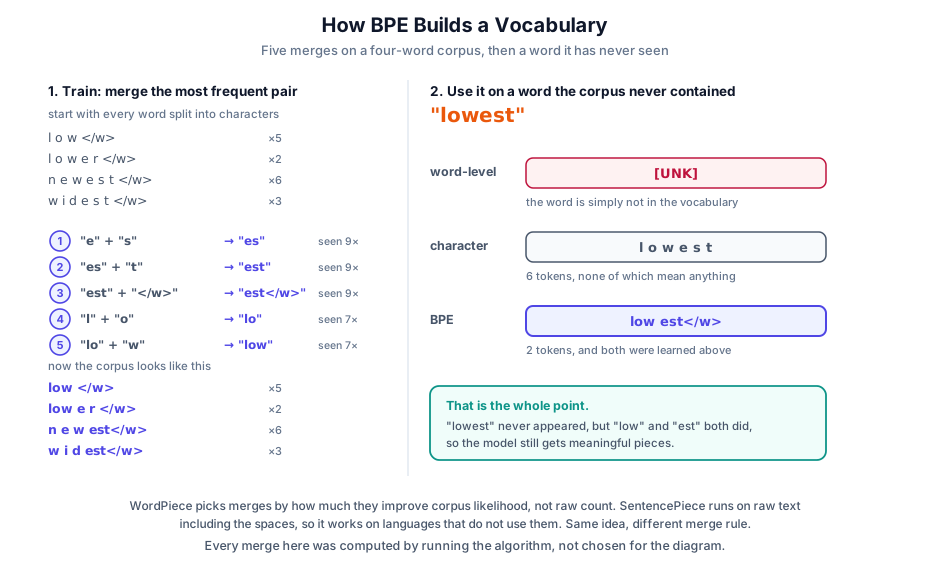
Follow the left column. The corpus is four words, every word starts as loose characters, and the algorithm just keeps merging whatever pair it sees most. After five merges “est” and “low” have both become single tokens, because they earned it.
Now the right column, which is the actual payoff. The word “lowest” never appears in that corpus. Word-level tokenization has nothing to offer but [UNK]. Character-level gives you six tokens that individually mean nothing. BPE gives you low + est, two pieces it learned separately, and the model can make sense of a word it has genuinely never seen.
Say it like this: BPE learns the common chunks, so a new word is just old chunks in a new order. Run it long enough and “ing” becomes one token because it’s everywhere, while a rare surname stays in pieces. GPT models use a byte-level variant, so any possible input encodes without a true unknown token.
WordPiece (BERT) does nearly the same, but chooses merges by how much they improve the likelihood of the corpus rather than by raw frequency. SentencePiece treats the raw string including spaces as the input, so it works on languages that don’t put spaces between words.
Why this matters more than it looks:
- An LLM struggles to count letters in a word because it never sees letters, it sees chunks.
- Arithmetic is shaky partly because numbers tokenize inconsistently.
- Non-English text often costs 2 to 3 times more tokens for the same meaning, which is a real bill.
Trap: “why can’t the model spell?” Because “strawberry” might be three tokens and none of them is a letter. The model isn’t stupid, it’s looking at a different alphabet to the one you are.
5. Dense Embeddings: Meaning as a Direction
Counting methods give you a vector that is enormous, mostly empty, and semantically blind. What if the vector was small, dense, and learned so that similar words end up near each other?
Say it like this: an embedding is a word’s coordinates, learned so that words used in similar ways land in similar places.
5.1 word2vec
Built for: giving every other NLP model better input. By 2013 everyone had classifiers and taggers that worked; they were all being fed sparse count vectors that knew nothing.
The trick is to learn meaning without anyone labelling anything, using a bet: words that show up in the same contexts mean similar things. Train a model on a fake task and keep the by-product.
Two flavours:
| Flavour | The fake task | Better at |
|---|---|---|
| CBOW | given the surrounding words, guess the middle one | faster, better on frequent words |
| Skip-gram | given a word, guess its neighbours | slower, better on rare words |
Nobody wants the predictions. You throw the model away and keep the weight matrix, and those rows are your embeddings.
The famous demonstration is that directions carry meaning:
$$\text{king}-\text{man}+\text{woman}\approx\text{queen}$$That’s not a trick. “Maleness” ended up as an actual direction in the space, because the training data used those words in systematically offset contexts.
5.2 GloVe and fastText
GloVe gets there differently: instead of sliding a window and predicting, it builds the global co-occurrence matrix for the whole corpus and factorizes it. Counting and prediction turn out to be two routes to nearly the same place.
fastText fixes the unknown-word hole by embedding character n-grams as well as whole words. “unhappiness” gets a vector even if it never appeared, because “un”, “happi” and “ness” all did.
5.3 The flaw that ended this era
Every method above gives each word exactly one vector, for all time.
I sat on the river bank. I withdrew cash from the bank.
Same vector. The model has averaged two unrelated meanings into one point in space, and it has no mechanism to ever tell them apart, because it never looks at the sentence.
Say it like this: static embeddings give a word one meaning, but words don’t have one meaning.
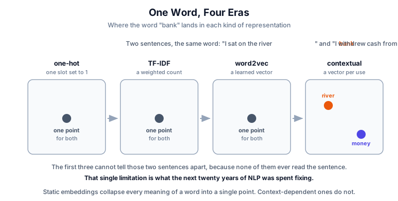
Fixing that needs a vector that depends on the words around it. Which means something has to read the sentence.
5.4 ELMo, the missing link
The first widely used answer wasn’t a transformer. ELMo ran a deep bidirectional LSTM language model over the sentence and used its internal states as the embeddings.
Say it like this: ELMo was word2vec that read the sentence first.
Same word, different sentence, different vector. It jumped the state of the art across a spread of tasks almost overnight and made one thing obvious to everyone: contextual beats static, and the remaining question was only what should do the reading. Transformers answered that within a year.
6. Reading the Sentence: RNNs
Built for: anything where order matters. Language modelling, tagging each word with its part of speech, speech recognition.
Process words one at a time, and carry a running summary as you go.
Say it like this: an RNN reads left to right and keeps a note of what it has seen so far.
$$h_t=f(W h_{t-1}+U x_t)$$That single line is the whole idea: the new state depends on the previous state and the current word. It handles any length, and the same weights get reused at every step.
What breaks: the same thing that breaks any deep stack, because unrolled over 50 words this is a 50-layer network. Multiply the same derivative fifty times and the gradient either vanishes or explodes (the mechanism is in the activation post). In practice a plain RNN forgets the start of a long sentence.
6.1 LSTM and GRU
The LSTM adds a separate cell state that runs alongside the hidden state, and three gates that decide what to forget, what to add, and what to output.
Say it like this: the LSTM adds a conveyor belt that information can ride along untouched, plus gates that decide what gets on and off.
The point is that conveyor belt. The cell state is mostly added to rather than multiplied through, so the gradient has a path backward that doesn’t get squeezed at every step. That’s the fix for forgetting.
GRU does a similar job with two gates instead of three and no separate cell state. Fewer parameters, trains faster, usually within noise of the LSTM.
Pros: genuinely handles context, still fine for short sequences and small data. Cons: the one that killed it. You cannot parallelize across time. Step 50 needs step 49 finished. When your competitor can process the whole sentence at once on a GPU, this is not a close race.
7. seq2seq and the Bottleneck
Built for: machine translation, very specifically. This is the architecture behind the first neural Google Translate.
To translate, you need variable input and variable output. seq2seq uses two RNNs: an encoder reads the source and compresses it into a final hidden state, and a decoder generates from that state.
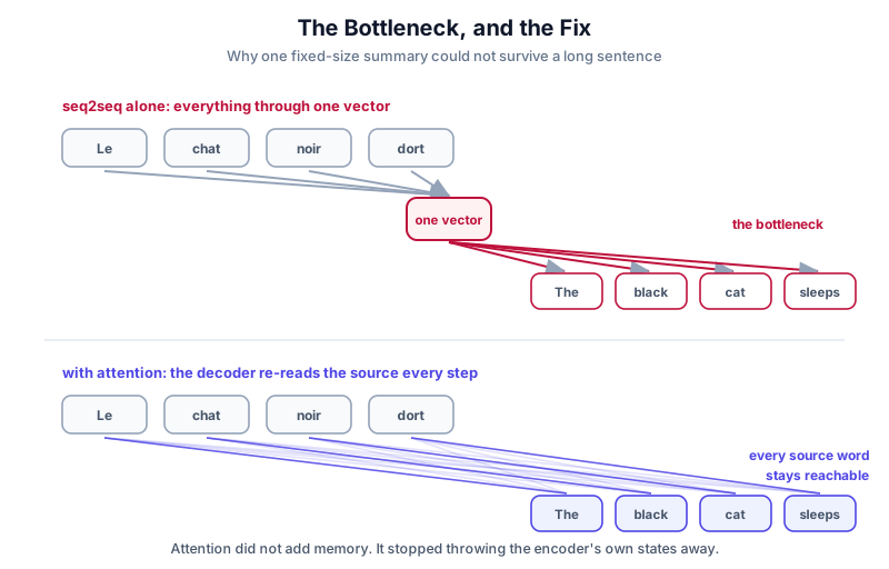
The flaw is visible the moment you draw it. The entire source sentence, however long, has to fit through one fixed-size vector. Translation quality was fine on short sentences and fell off a cliff as they got longer, which is exactly what you’d predict from a fixed-size summary.
Say it like this: seq2seq made the encoder write a one-sentence summary and then hid the original from the decoder.
7.1 Attention, 2014
Built for: the same job, done better. The paper is literally called Neural Machine Translation by Jointly Learning to Align and Translate, and alignment means working out which source word each output word corresponds to.
The fix, from Bahdanau and colleagues, is almost embarrassingly direct: stop throwing the encoder states away. Keep all of them, and let the decoder look back at the whole source each time it produces a word, deciding for itself which source words matter right now.
Say it like this: instead of one summary, the decoder gets to re-read the source and highlight what it needs.
Two scoring flavours you should recognize by name:
| How it scores a match | Cost | |
|---|---|---|
| Bahdanau (additive) | a small learned network over the pair | slower, more expressive |
| Luong (multiplicative) | a dot product, optionally with a matrix | faster, and what won |
This worked so well that a reasonable question followed: if attention is doing the heavy lifting, what exactly is the RNN still for?
8. The Transformer: Drop the Recurrence
Built for: translating faster. Attention Is All You Need is a machine translation paper; its headline result is a BLEU score. That it would end up running everything from chatbots to protein folding was not the pitch.
The 2017 answer was to delete the RNN and keep only attention.
Say it like this: the transformer replaced “read the words in order” with “let every word look at every other word at once”.
That single change buys the thing that mattered most: the whole sequence processes in parallel on a GPU. No waiting for step 49.
8.1 Self-attention, and what Q, K and V actually are
Every word produces three vectors by multiplying its embedding by three learned matrices. The names are less mysterious than they look if you think about what each one is for:
- Query is what this word is looking for.
- Key is what this word offers, an advertisement.
- Value is what this word actually hands over if you pick it.
Say it like this: every word writes a search query, an advert, and a payload. Attention matches queries against adverts, then adds up the payloads.
The mechanism is four steps, and you can do it by hand:
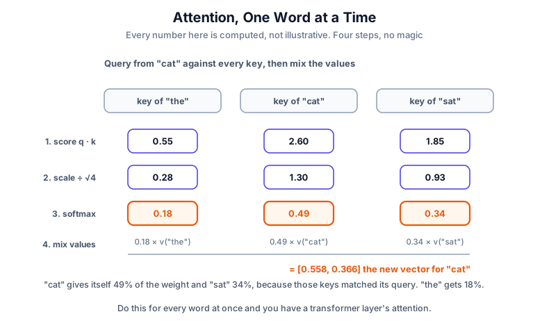
Those numbers are computed, not decorative. “cat” ends up giving 49% of its attention to itself and 34% to “sat”, because those two keys matched its query. “the” gets 18% and contributes almost nothing. Do that for every word simultaneously and you’ve done a transformer layer’s attention.
- Score. Dot every query with every key. A big dot product means that key is relevant to that query.
- Scale. Divide by \(\sqrt{d_k}\).
- Softmax. Turn the scores into weights that sum to 1.
- Mix. Add up the value vectors, weighted by those numbers.
All of it, for the whole sequence at once:
$$\text{Attention}(Q,K,V)=\text{softmax}\!\left(\frac{QK^{T}}{\sqrt{d_k}}\right)V$$Trap: “why divide by \(\sqrt{d_k}\)?” Dot products of \(d_k\)-dimensional vectors grow with \(d_k\), so with a 64-dimensional head the raw scores are large, softmax saturates, and you get a nearly one-hot distribution with almost no gradient. Dividing by \(\sqrt{d_k}\) holds the variance near 1 and keeps softmax in its useful range. Saying “it stops softmax saturating” is the answer; saying “for stability” is the memorized one.
8.2 Multi-head attention
One attention operation produces one weighted average, which means one opinion about what relates to what. Language has several kinds of relationship at once: what the verb is, what the pronoun refers to, which adjective belongs to which noun.
Say it like this: one head can only have one opinion, so you run several and let them specialize.
Split the model dimension into \(h\) heads, run attention in each independently, concatenate the results, and pass them through one more matrix. With \(d_{model}=512\) and 8 heads, each head works in 64 dimensions, so the total cost is roughly the same as one big head.
Cons worth knowing: heads are not interpretable by default (the tidy “this head does coreference” pictures are cherry-picked), and a decent fraction of heads in a trained model turn out to be prunable.
8.3 Inside one block
Attention is only half a layer. The full block wraps it in machinery that exists purely to make deep stacks trainable.
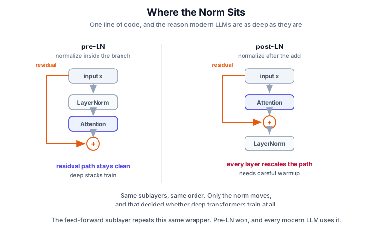
Where that norm sits turns out to matter enormously, and §11.3 comes back to it.
- Residual connections around each sublayer. The output is \(x + \text{Sublayer}(x)\), so there’s a path the gradient can travel backward without passing through anything that shrinks it.
- Normalization to keep activations in a sane range.
- A feed-forward network applied to each position separately: expand to roughly 4x the width, apply a nonlinearity, project back. This is where most of the parameters live, and it’s the layer’s chance to actually compute something rather than just move information around.
Say it like this: attention moves information between positions, the feed-forward layer thinks about it, and the residuals make sure the gradient survives the trip.
One piece sits outside the stack: the LM head, the final matrix that turns the last layer’s vector into one score per vocabulary entry. With a 128,000-token vocabulary and 4,096 dimensions that single matrix is over 500 million parameters, which is why many models tie it to the input embedding matrix and use one set of weights for both. Same table, read in both directions.
8.4 Positional encoding
Here’s an uncomfortable property. Attention computes a weighted average over a set. Shuffle the input words and the outputs shuffle with them, unchanged. The architecture has no idea what order anything came in.
Say it like this: attention sees a bag of words, not a sentence, unless you tell it where each word sits.
So you add position information to the embeddings before the first layer. The original paper used fixed sine and cosine waves at different frequencies; every position gets a distinct pattern, and the wave structure means relative offsets are expressible.
This is one of the most-revised parts of the architecture, and §11 covers where it went.
9. The Three Families
Every transformer you’ve heard of is one of three shapes, and the difference is entirely what each token is allowed to look at.
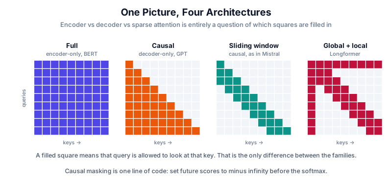
| Family | Attention pattern | Examples | Good at | Bad at |
|---|---|---|---|---|
| Encoder-only | every token sees every token | BERT, RoBERTa, embedding models | classification, NER, retrieval, anything where you have the whole text up front | generating text, which it was never built to do |
| Decoder-only | token \(t\) sees only tokens up to \(t\) | GPT, LLaMA, Mistral, Qwen | generation, and by now nearly everything else | it can’t look ahead, so its representation of a token never sees the rest of the sentence |
| Encoder-decoder | encoder bidirectional, decoder causal plus cross-attention to the encoder | T5, BART, most translation models | tasks with a distinct input and output: translate, summarize | roughly twice the machinery, and awkward to scale |
Say it like this: encoder-only reads, decoder-only writes, encoder-decoder reads one thing and writes another.
The interesting part is why decoder-only won. It’s not that causal attention is better at understanding, because it plainly isn’t. It’s that next-token prediction is a task you can run on any text in existence, one architecture then covers every task if you phrase the task as text, and one causal stack is simpler to scale than two towers. Uniformity beat specialization.
9.2 Two ways to compare two texts
If the job is “does this document match this query”, there are two architectures and the difference is a real design decision.
| How it works | Speed | Quality | |
|---|---|---|---|
| Bi-encoder | encode each text separately, compare the two vectors with cosine | you can embed the whole corpus once, offline. A query is one forward pass plus a vector search | good |
| Cross-encoder | feed the pair in together so every query token can attend to every document token | one forward pass per pair, so you cannot precompute anything | clearly better |
Say it like this: a bi-encoder reads the two texts separately and compares notes. A cross-encoder reads them side by side.
That extra attention between the two texts is exactly where the cross-encoder’s accuracy comes from, and exactly why it can’t scale. So production does both: a bi-encoder retrieves the top 100 from millions, then a cross-encoder reranks those 100. Fast filter, accurate finish.
Trap: “is BERT obsolete?” No, and saying so is a tell. For classification and especially for retrieval embeddings, a small bidirectional encoder is faster, cheaper, and often better than asking a 70B decoder. Plenty of production search stacks are still BERT-shaped.
10. How a Model Actually Writes a Sentence
Everything above describes one forward pass. But a forward pass gives you a score for every token in the vocabulary, not a sentence. Turning those scores into text is its own set of decisions, and they change the output more than most people expect.
Say it like this: the model never writes a sentence. It writes one token, sticks it on the end of the input, and runs again.
10.1 Two phases, not one
Generation splits into two very different jobs, and confusing them is why people get surprised by latency.
| Phase | What happens | Bottleneck |
|---|---|---|
| Prefill | your whole prompt goes through in one parallel pass | compute. Long prompts cost real FLOPs |
| Decode | one token at a time, each needing a full pass | memory bandwidth. You reread the weights for every single token |
That split is exactly why serving metrics come in pairs: time to first token is prefill, and time per output token is decode. They’re tuned differently because they’re limited by different hardware.
Decode is the awkward one. For each token you load the entire model’s weights out of memory to produce one word, which is why GPUs sit underused during generation, and why batching many requests together is the standard fix.
The KV cache is what keeps this from being much worse: keys and values for tokens already processed are stored, so each new token attends to the cache instead of recomputing everything. It’s also what MQA and GQA exist to shrink.
10.2 Picking the next token
The final layer gives you one score per vocabulary entry. Softmax turns those into probabilities. Now what?
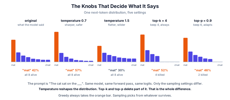
Greedy takes the highest-probability token, every time. Deterministic and reproducible, which is good, and prone to loops like “the the the”, which is not.
Beam search keeps the \(k\) most promising sequences rather than committing to one token, and picks the best complete one at the end. It genuinely helps when there is a roughly correct answer: translation, summarization, speech transcription.
Trap, and a good interview question: why doesn’t ChatGPT use beam search? Because beam search finds high-probability text, and high-probability text is boring. Humans don’t speak in maximum-likelihood sentences, they surprise you a bit. Optimize likelihood hard enough on open-ended generation and you get bland, repetitive, strangely lifeless output. For open-ended text, sampling beats searching.
Sampling draws from the distribution instead of maximizing it. Which needs shaping, and that’s what the knobs do.
| Knob | What it does | Typical |
|---|---|---|
| Temperature | divides the logits before softmax. Below 1 sharpens toward the top token, above 1 flattens toward uniform | 0.7 to 1.0 |
| Top-k | keep only the \(k\) highest-probability tokens, renormalize, sample | 40 to 50 |
| Top-p (nucleus) | keep the smallest set whose probabilities sum past \(p\) | 0.9 to 0.95 |
| min-p | keep tokens above a fraction of the top token’s probability | 0.05 to 0.1 |
| Repetition / frequency penalty | push down tokens already used | small, or zero |
Say it like this: temperature changes how confident the distribution looks, top-k and top-p decide how many options stay on the table.
The reason top-p beat top-k in practice is that it adapts. When the model is certain (after “the capital of France is”) a good distribution has one obvious winner, and top-k still forcibly keeps 40 candidates including nonsense. Top-p keeps just the one. When the model is genuinely unsure, top-p widens out on its own.
Trap: “temperature 0” is not really a temperature, it’s a division by zero. Every framework special-cases it to mean greedy. And temperature 0 still isn’t perfectly reproducible on GPU, because floating-point reduction order varies with batching.
10.3 Speculative decoding
Since decode is limited by memory bandwidth rather than compute, there’s spare arithmetic going begging. Speculative decoding spends it: a small fast model drafts several tokens, then the big model checks them all in one parallel pass and keeps the ones it agrees with.
Say it like this: a cheap model guesses ahead and the expensive model marks the homework, several tokens at a time.
Because verification is parallel, you get several tokens for roughly the cost of one. The output is identical to what the big model would have produced alone, which is the part that makes it free rather than a tradeoff.
11. The Parts You Can Swap
This is where architectures actually differ in 2026. Each of these is a fix for a specific cost of the vanilla transformer.
11.1 Attention variants
Self vs cross. In self-attention, Q, K and V all come from the same sequence. In cross-attention, the queries come from one sequence and the keys and values from another, which is how a decoder reads an encoder.
Causal masking is not a different mechanism, just a mask. Set every score for a future position to \(-\infty\) before the softmax and it gets zero weight. That one line is the entire difference between BERT-style and GPT-style attention.
The KV cache problem. When generating, you don’t recompute keys and values for tokens you’ve already processed, you cache them. That cache grows with every token, and for long contexts it gets larger than the model weights. Which is what the next two variants are for.
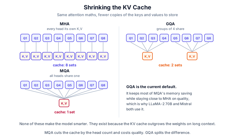
| Variant | K/V heads | KV cache | Quality |
|---|---|---|---|
| MHA (original) | one per query head | biggest | the reference |
| MQA | one, shared by all heads | smallest, cut by the head count | measurably worse |
| GQA | one per small group of heads | middle | close to MHA |
Say it like this: MQA makes all the heads share one set of keys and values, GQA lets small groups share, and both exist to shrink the cache rather than to think better.
GQA is the current default (LLaMA-2 70B, Mistral) because it gets most of MQA’s memory saving with little of its quality loss.
Sliding window attention attacks the other cost: the quadratic one. Let each token attend only to the \(w\) tokens nearest it, and cost falls from \(O(n^2)\) to \(O(n\cdot w)\). Stack enough layers and information still travels far, the same way a CNN’s receptive field grows with depth, just indirectly.
Sparse and global-local patterns (Longformer) keep a sliding window for most tokens and let a few special tokens attend to everything, so there’s still a global channel.
Linear attention (Performer, Linformer) approximates the softmax so the whole thing becomes \(O(n)\). It works, and it consistently costs quality, which is why it stayed niche.
Trap, and a good one: FlashAttention is not an attention variant. It computes exactly the same numbers as standard attention. What it changes is memory traffic: it tiles the computation so the \(n\times n\) score matrix is never written to GPU main memory at all. Same maths, several times faster, much less memory. Calling it an approximation is a giveaway that you’ve only read the name.
11.2 Positional encoding variants
Each of these fixes the previous one’s failure to handle sequences longer than it trained on.
| Scheme | How | Cost |
|---|---|---|
| Sinusoidal | fixed sine/cosine waves added to the embedding | no parameters, but the model doesn’t really extrapolate |
| Learned absolute | an embedding per position (BERT, GPT-2) | simple, and hard-capped at the trained length |
| Relative | encode the distance between tokens, not their absolute slots (T5) | generalizes better, more expensive |
| RoPE | rotate Q and K by an angle proportional to position | relative by construction, plays nicely with the KV cache, extends with tricks. The modern default |
| ALiBi | add a distance-proportional penalty straight onto the attention scores | no position embeddings at all, strong extrapolation |
Say it like this: absolute positions tell a token where it sits, relative ones tell it how far away everything else is, and the second generalizes because distance still means something past the training length.
RoPE is what LLaMA and most modern open models use. The reason is worth understanding: because it rotates rather than adds, the dot product between two rotated vectors depends only on their difference in position. You get relative behaviour without computing a relative bias for every pair.
11.3 Normalization variants
Post-LN vs pre-LN is a one-line change that decided whether very deep transformers train at all.
The original paper normalized after the residual add. Deep post-LN models are unstable and need careful warmup. Move the norm inside the residual branch, so the skip path stays untouched all the way down, and suddenly deep stacks train. Every modern LLM is pre-LN.
Say it like this: pre-LN keeps the residual highway clean, and that’s what let models get deep.
RMSNorm drops the mean-subtraction and the bias from LayerNorm and only rescales by the root-mean-square. Cheaper, one fewer statistic to compute, and empirically just as good. Used in LLaMA and most things since.
11.4 Feed-forward variants
The FFN is where most parameters live, so it’s where people look for gains.
The original was linear → ReLU → linear. BERT and GPT moved to GELU. Modern LLMs mostly use SwiGLU, a gated variant where one projection produces the signal and another produces a gate that multiplies it (the activation post covers why gating helps and the 2/3 width adjustment).
Mixture of Experts is the bigger structural change. Replace the single FFN with \(N\) expert FFNs plus a small router, and send each token to only the top \(k\) of them.
Say it like this: MoE gives the model far more parameters than it uses on any one token.
Mixtral runs 8 experts with top-2 routing, so it holds roughly 47B parameters and spends about 13B per token.
Pros: capacity grows without the FLOPs growing with it. Cons: you still have to hold all the experts in memory, routing can collapse onto a few favourites without a balancing term, and distributed serving gets genuinely harder.
11.5 The alternative to attention entirely
Attention’s cost is structural: every token looks at every token. State space models go back to a recurrence, but one designed so it can also be computed as a convolution, which means it trains in parallel like a transformer and runs like an RNN.
Mamba adds selectivity: the recurrence parameters depend on the input, so the model can decide what to keep and what to drop rather than applying a fixed filter.
Say it like this: attention keeps every token and can look any of them up. An SSM keeps a fixed-size summary and can’t.
Pros: linear in sequence length, and inference memory is constant instead of a KV cache that grows forever. Cons: that fixed-size state is a real ceiling. Tasks that need exact recall of something specific from far back (copying, retrieval, “what was the number in paragraph three”) are exactly where attention’s ability to look anything up wins. Which is why most practical systems are hybrids rather than pure SSMs.
12. What’s Still Broken
Every section above ended with something the next idea fixed. These are the ones nothing has fixed yet, and they’re the honest answer when an interviewer asks about limitations.
| Problem | Why it’s structural |
|---|---|
| Quadratic attention | every token looking at every token is the mechanism. Sliding windows and linear attention are workarounds that give something up |
| Lost in the middle | a long context window is not the same as using it. Models reliably attend to the start and the end and get vague about the middle |
| KV cache growth | linear in context length, and on long conversations it outgrows the weights. GQA shrinks the constant, not the growth |
| Position extrapolation | even RoPE degrades well before the advertised limit. “128k context” is a capacity, not a promise of quality |
| Hallucination | next-token prediction optimizes for plausible, and plausible and true are different objectives. Nothing in the architecture checks facts |
| No memory | the context window is the only memory there is. Every conversation starts from nothing |
| Tokenization leaks | counting letters, arithmetic, and the cost of non-English text all trace back to the chunking |
| Interpretability | we cannot say why a specific token was produced, only that the weights produced it |
Two of these deserve a sentence more.
Hallucination is not a bug that will be patched. The model was built to continue text convincingly. A fluent wrong answer and a fluent right answer look identical to the objective it optimizes. Retrieval and tool use work around it by supplying facts from outside the weights; nothing inside the architecture distinguishes true from plausible.
Long context is oversold. Context length is quoted like RAM, as though a 200k window means 200k tokens of reliable attention. In practice accuracy sags in the middle of long inputs, which is why retrieval still matters even when everything would technically fit.
Say it like this: the architecture is very good at producing text that sounds right, and it has no separate mechanism for checking whether it is right.
13. Rapid-Fire Q&A
Why did attention replace RNNs? Not accuracy, parallelism. An RNN has to finish step 49 before starting step 50, so it can’t use a GPU properly. Attention processes every position at once.
What are Q, K and V? A query is what a token wants, a key is what it advertises, a value is what it passes on. Score queries against keys, softmax, use the weights to average the values.
Why divide by \(\sqrt{d_k}\)? Dot products grow with dimension. Without the scaling, softmax saturates and gradients nearly vanish.
Why multiple heads? One attention pass produces one weighted average, so one notion of what relates to what. Several heads let the model track different relationships at once.
Encoder-only, decoder-only, or encoder-decoder? Reading tasks and embeddings, encoder. Generation, decoder. Distinct input and output like translation, encoder-decoder. Decoder-only dominates because one uniform architecture scales.
What is the KV cache and why do you care? Cached keys and values for tokens already generated, so you don’t recompute them. It grows with every token and on long contexts it outgrows the model weights, which is why MQA and GQA exist.
MQA vs GQA? MQA shares one set of K/V across all heads: smallest cache, real quality cost. GQA shares within small groups: nearly MHA quality, most of the saving. GQA is the default.
Is FlashAttention an approximation? No. Identical outputs, reordered to avoid writing the \(n\times n\) matrix to GPU memory.
Why RoPE over learned positions? Learned absolute positions cannot go past the length they trained on. RoPE rotates Q and K so attention depends on the difference in positions, which still means something further out.
Pre-LN or post-LN? Pre-LN. It keeps the residual path clean and is why deep transformers train without elaborate warmup schedules.
Is TF-IDF still worth knowing? Yes. It’s the twenty-minute baseline that occasionally wins, and it tells you whether the problem was ever hard.
Why can’t LLMs count letters? Tokenization. They see subword chunks, not characters, so the letters aren’t individually visible.
What does an SSM give up compared to attention? Exact lookup. A fixed-size state can’t reach back and retrieve an arbitrary earlier token the way attention can.
Bi-encoder or cross-encoder? Bi-encoder to retrieve, because you can embed the corpus offline and a query is then one forward pass plus a vector search. Cross-encoder to rerank the shortlist, because letting the two texts attend to each other is worth real accuracy but costs a forward pass per pair.
What was ELMo and why does it matter? A deep bidirectional LSTM language model whose internal states were used as embeddings. It was the first widely used contextual embedding and it proved contextual beats static, a year before BERT.
How does a model actually emit a word? The LM head, a matrix from the hidden size to the vocabulary size, gives one score per token, then softmax. It’s often tied to the input embedding matrix because otherwise it’s hundreds of millions of parameters on its own.
Why not beam search for chat? Beam search maximizes likelihood, and the most likely text is bland and repetitive. Humans don’t talk in maximum-likelihood sentences. Beam still wins where there is a correct answer, like translation.
Temperature vs top-p? Temperature reshapes the whole distribution, sharper below 1 and flatter above. Top-p truncates it, keeping the smallest set of tokens that covers \(p\) of the mass. They stack, and top-p is preferred over top-k because it adapts to how confident the model is.
Why is the first token slow and the rest fast? Prefill processes your entire prompt in one parallel pass, so it’s compute-bound. Decode emits one token at a time and rereads the weights each time, so it’s memory-bound. That’s TTFT against TPOT.
What is speculative decoding? A small model drafts several tokens, the big model verifies them in one parallel pass. Same output as the big model alone, fewer sequential passes.
Why do LLMs hallucinate? Next-token prediction optimizes plausibility. A fluent wrong answer scores the same as a fluent right one, and nothing in the architecture checks facts.
Does a 200k context window mean 200k usable tokens? No. Accuracy degrades in the middle of long inputs, which is why retrieval still matters even when everything fits.
The Idea Underneath
Every step in this post is the same move: someone found what the current representation was throwing away, and built the next thing to stop throwing it away.
One-hot threw away meaning, so embeddings learned it. Embeddings threw away context, so RNNs read the sentence. RNNs threw away parallelism, so attention removed the recurrence. Attention throws away nothing, which is precisely why it costs \(O(n^2)\), and every variant since is an argument about what you’re willing to throw away again to get that cost back down.
And the four jobs from the start never changed. People still want to find the right document, guess the next word, turn one sequence into another, and label some text. What changed is that one architecture now does all four, which is a genuinely strange outcome given that it was designed to translate German a bit faster.
That’s the field, and it’s why the chain is worth knowing in order. When the next architecture appears, the useful question isn’t what it does. It’s what did it decide to stop keeping.