Third in a series with loss functions and activation functions. The loss defines what “good” means. The activation decides what the network can express. The optimizer is what actually gets you there, and it is where most training runs are won or lost.
1. The 60-Second Table
| Optimizer | The idea in one line | Extra memory | Use it for |
|---|---|---|---|
| SGD | Step downhill | none | Convex problems, classic vision with tuning |
| SGD + Momentum | Keep a running velocity | 1x params | ResNets, anything where SGD works |
| Nesterov | Momentum that looks ahead | 1x params | A small free improvement on momentum |
| AdaGrad | Per-parameter step from total past gradient | 1x params | Sparse features. Historical |
| RMSProp | Same, but a decaying average | 1x params | RNNs. Mostly superseded |
| Adam | Momentum plus RMSProp, bias corrected | 2x params | The strong baseline for deep nets |
| AdamW | Adam with decoupled weight decay | 2x params | Transformers. The real default |
| Lion | Sign of momentum only | 1x params | Large models, when memory is tight |
| Sophia | Clipped diagonal second-order | 2x params | LLM pretraining, faster convergence |
| Shampoo / SOAP | Matrix preconditioner | 4x+ params | Large runs where the math pays off |
| Muon | Orthogonalized momentum on weight matrices | 1x params | Emerging large-model optimizer |
If you remember one thing: use AdamW with warmup and cosine decay, and spend your tuning budget on the learning rate, not on the optimizer. The choice of optimizer is worth a few percent. The learning rate is worth the difference between a working model and a nan.
2. What Optimization Actually Is
You have a loss \(L(\theta)\) and you want the parameters that minimize it:
$$\theta^* = \arg\min_\theta L(\theta)$$For linear regression there is a closed form. For a neural network with a billion parameters there is not, so you do the only thing available: start somewhere, compute which direction is downhill, take a step, repeat.
$$\theta_{t+1} = \theta_t - \eta\nabla_\theta L(\theta_t)$$That is gradient descent, and everything in this post is a variation on deciding how big a step and in what direction.
The high-dimensional intuition that matters. Beginners worry about local minima. In a billion-dimensional space, a local minimum requires the loss to curve upward in every one of a billion directions at once, which is vanishingly unlikely. What you actually hit are saddle points, where some directions go up and others go down, and vast flat plateaus where the gradient is tiny and progress stalls. Most optimizer design is about escaping flatness and noise, not about climbing out of bowls.
Trap: “how do you avoid local minima?” is a question with an outdated premise. The strong answer names the premise: in high dimensions saddle points and plateaus are the real obstacle, and SGD’s gradient noise is one of the things that helps escape them.
Where the Gradient Comes From
Everything above assumes you have \(\nabla L\). Backpropagation is how you get it, and the most useful thing to be precise about is the division of labor:
Backprop computes the gradient. The optimizer decides what to do with it. They are separate stages, and swapping Adam for SGD changes nothing about how the gradient was produced.
What it actually is: reverse-mode automatic differentiation, which is the chain rule applied in a particular order. The forward pass builds a graph of operations and caches intermediate values. The backward pass walks that graph in reverse, multiplying local derivatives as it goes, until every parameter has a partial derivative.
Here is the whole mechanism on a graph small enough to check by hand:
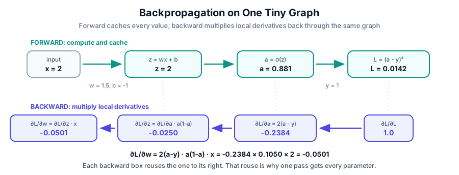
Follow the bottom row right to left. Each box takes the gradient handed to it from the right and multiplies by one local derivative, something each operation knows about itself without knowing anything about the rest of the network: the squared error knows \(2(a-y)\), the sigmoid knows \(a(1-a)\), the linear layer knows \(x\). Multiply them and you get \(\partial L/\partial w = -0.0501\).
That locality is the trick. No operation needs a global view; it only needs its own derivative and whatever arrived from downstream. Which is why the same machinery works on a three-node graph and on a 500-billion-parameter transformer without changing.
Why reverse and not forward? This is the part worth understanding, because it is the reason deep learning is computationally possible at all. You have \(N\) parameters and exactly one scalar loss.
| Mode | Cost scales with | For a network |
|---|---|---|
| Forward-mode AD | number of inputs | \(N\) passes, one per parameter. Hopeless |
| Reverse-mode AD | number of outputs | one pass, since the loss is a single scalar |
One backward pass recovers all \(N\) partial derivatives for roughly the cost of one forward pass. That asymmetry is the whole game, and it is why the algorithm runs backward.
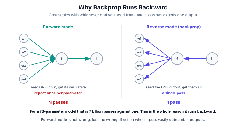
Both directions compute exactly the same derivatives. The difference is how many sweeps you need: seeding from the input side gets you one parameter’s derivative per sweep, while seeding from the output side gets you all of them at once, because there is only one output to seed. With four weights that is a 4x difference. With seven billion it is the difference between training a model and not.
The catch is memory: reverse mode must keep the forward activations until backward consumes them, because the local derivatives are computed at those values. Forward mode needs no such tape. That tradeoff is not academic, and it is exactly the cost that gradient checkpointing exists to buy back.
Two consequences that echo through the rest of this post:
- Backward needs the cached forward pass, so activations are a first-class memory cost, often the largest one.
- The chain rule is a product of local derivatives, so long chains multiply many numbers together. If those numbers are below 1 the gradient vanishes; above 1 it explodes. That is the same product argument as the activation functions post, and it is why the choice of activation and the choice of initialization are optimization concerns, not just architecture ones.
Trap: “is backpropagation an optimization algorithm?” No. It is a differentiation algorithm. Gradient descent is the optimizer; backprop is what hands it the gradient. A related one: “backprop” and “autograd” are not competing things. Autograd is the framework’s implementation of reverse-mode AD, which is backprop generalized to an arbitrary graph.
In practice you rarely write it yourself, but you do control it: loss.backward() populates .grad, torch.no_grad() skips building the graph for inference, .detach() cuts a tensor out of it, and zero_grad() matters precisely because gradients accumulate rather than overwrite, which is the mechanism gradient accumulation exploits on purpose.
Batch, Stochastic, Mini-batch
| Variant | Gradient from | Per step | Reality |
|---|---|---|---|
| Batch GD | the entire dataset | exact, slow | Unusable past toy sizes |
| SGD | one example | very noisy, fast | Too noisy in practice |
| Mini-batch | 32 to millions of tokens | the useful middle | What everyone actually does |
Everyone says “SGD” and means mini-batch. Nobody is doing one example at a time.
The noise is not just a cost you tolerate. Gradient noise helps you skid past saddle points and acts as an implicit regularizer, which is a large part of why small-batch SGD often generalizes better than a very large batch, and why simply cranking the batch size up does not give you a free win.
3. Momentum: The First Real Fix
Plain gradient descent has an ugly failure mode. When the loss surface is a long narrow valley, steep across and shallow along, the gradient points mostly across the valley rather than down it. You bounce between the walls and crawl toward the minimum.
Momentum accumulates a velocity instead of following each gradient blindly:
$$v_{t+1} = \beta v_t + \nabla L(\theta_t), \qquad \theta_{t+1} = \theta_t - \eta v_{t+1}$$With \(\beta=0.9\), roughly the last ten gradients are averaged. The oscillating across-valley components cancel out while the consistent down-valley component accumulates. You stop bouncing and start rolling.
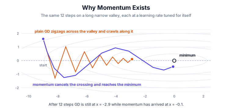
Both runs get twelve steps and each uses a learning rate tuned for itself, so this is not a rigged comparison. Plain GD is already at the largest step it can take without diverging in the steep direction, and it spends that budget bouncing between the walls: after twelve steps it has crawled from \(x=-9\) to only \(x=-2.9\). Momentum’s velocity term cancels the alternating across-valley components and reaches \(x=-0.1\) in the same twelve steps.
Nesterov momentum evaluates the gradient after the momentum step rather than before, so it can correct an overshoot in the same update instead of the next one. It is a small, nearly free improvement: nesterov=True.
4. Adaptive Methods
Momentum fixes the direction. The other half of the problem is the step size, and specifically that one global learning rate has to serve every parameter, including a word embedding that fires on 0.01% of batches and a layer-norm gain that gets a gradient every step.
4.1 AdaGrad
Give every parameter its own step size, scaled down by how much that parameter has been updated so far:
$$G_t = G_{t-1} + g_t^2, \qquad \theta_{t+1} = \theta_t - \frac{\eta}{\sqrt{G_t}+\epsilon}g_t$$Rare features get large steps, frequent features get small ones. That was a genuine breakthrough for sparse problems.
The flaw is in the first line: \(G_t\) only ever accumulates. The denominator grows without bound, so the effective learning rate decays monotonically to zero and training stalls before convergence, whether or not you are done.
4.2 RMSProp
Same idea, one character different: replace the running sum with a running average.
$$E[g^2]_t = \rho E[g^2]_{t-1} + (1-\rho)g_t^2$$Now old gradients decay out of the estimate, the denominator stops growing forever, and the learning rate can recover when the landscape changes. This is AdaGrad’s fix, and it is the second half of Adam.
4.3 Adam
Adam is momentum and RMSProp at the same time: a running average of the gradient (first moment) and of its square (second moment).
$$m_t = \beta_1 m_{t-1} + (1-\beta_1)g_t, \qquad v_t = \beta_2 v_{t-1} + (1-\beta_2)g_t^2$$$$\hat m_t = \frac{m_t}{1-\beta_1^t}, \qquad \hat v_t = \frac{v_t}{1-\beta_2^t}, \qquad \theta_{t+1} = \theta_t - \eta\frac{\hat m_t}{\sqrt{\hat v_t}+\epsilon}$$Defaults \(\beta_1=0.9\), \(\beta_2=0.999\), \(\epsilon=10^{-8}\) work across an astonishing range of problems, which is most of why Adam took over.
Why bias correction exists. \(m\) and \(v\) start at zero, so early on they are biased toward zero, and \(v\) being too small would produce enormous steps exactly when the model is most fragile. Dividing by \(1-\beta^t\) undoes that. Note \(\beta_2^t\) with \(\beta_2 = 0.999\) takes thousands of steps to decay, which is precisely why the first few thousand steps of Adam are delicate and why warmup exists.
Trap: “what are Adam’s two moments?” Not “mean and variance.” The first moment is the mean of the gradient, the second is the mean of the gradient squared, which is the uncentered second moment. It is only the variance if the mean is zero.
4.4 AdamW, and Why It Matters
This is the most consequential small detail in modern training, and it connects straight back to L2 regularization in the loss post.
Adding an L2 penalty to the loss puts \(\lambda\theta\) into the gradient. Adam then divides that whole gradient by \(\sqrt{\hat v}\). So a parameter with large historical gradients gets its weight decay divided down too, and the regularization you thought you configured is quietly applied unevenly across the network.
AdamW decouples them. The decay is applied directly to the weights, outside the adaptive machinery:
$$\theta_{t+1} = \theta_t - \eta\frac{\hat m_t}{\sqrt{\hat v_t}+\epsilon} - \eta\lambda\theta_t$$That last term is the entire difference, and it is worth real accuracy on transformers. torch.optim.AdamW is the right default. If you see Adam(weight_decay=0.01) in a transformer codebase, that is a bug worth raising.
Trap: “L2 regularization and weight decay are the same thing.” True for plain SGD, false for any adaptive optimizer. That distinction is the whole reason AdamW exists.
5. Learning Rate: The Hyperparameter That Actually Matters
You can swap optimizers and move a few percent. Get the learning rate wrong by 10x and you get divergence or a model that never trains.
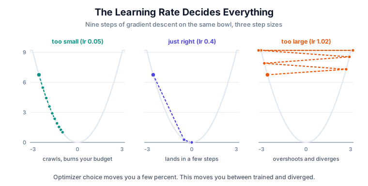
Note the third panel: the learning rate is 1.02, barely above the stability threshold of 1.0 for this bowl. A 2% change is the difference between converging and diverging. That is the actual sensitivity you are dealing with, and it is why an LR sweep is worth more than an optimizer sweep.
Warmup. Start near zero and ramp up over the first few hundred to few thousand steps. Two reasons, and the good answer gives the second: early gradients are large and unrepresentative, and Adam’s second-moment estimate \(\hat v\) is built from very few samples early on, so it is high variance, so the adaptive denominator is unreliable exactly when a bad step does the most damage. Warmup buys time for \(v\) to become meaningful.
Decay. Once you are converging, large steps stop helping and start bouncing you around the minimum. The standard options:
| Schedule | Shape | Where you see it |
|---|---|---|
| Cosine | smooth ramp down to ~0 | The default for most pretraining |
| Linear | straight line down | BERT-style finetuning |
| Step | drop 10x at milestones | Classic vision, ResNet recipes |
| WSD | warmup, long constant, short sharp decay | Modern LLM runs, lets you stop anywhere |
Warmup-stable-decay deserves a mention because it solves a real operational problem: with cosine you must fix the total step count in advance, since the shape depends on where the end is. WSD holds a constant rate for as long as you like and only decays at the end, so you can decide to stop later without invalidating the schedule.
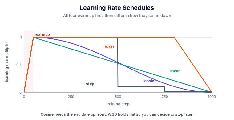
The shaded strip at the left is warmup, common to all four. Look at the difference in shape after that: cosine and linear both start decaying immediately and their entire path depends on knowing the final step count, while WSD spends most of training at the full rate and only pays the decay at the end. That is why WSD lets you extend a run without invalidating the schedule you already trained under.
Batch size and learning rate move together. The linear scaling rule says that when you multiply batch size by \(k\), multiply the learning rate by \(k\) as well, with warmup to survive the start. The intuition: a batch \(k\) times larger gives a gradient estimate with lower variance, so you can afford to trust it proportionally more. It holds well up to a point and then breaks down, which is where large-batch training gets genuinely hard.
Trap: “you changed batch size and the model got worse, why?” Because you changed the effective learning rate without meaning to. This is the single most common cause of “it worked on my machine, then we scaled it up.”
6. The Modern Frontier
Adam has held the crown for a decade. What is challenging it, and why:
Lion (2023) keeps only momentum and uses the sign of the update, discarding magnitude. That halves optimizer memory versus Adam and works surprisingly well at scale. It needs a smaller learning rate and larger weight decay than Adam, which trips people up on first use.
Sophia uses a cheap clipped estimate of diagonal curvature, a light-touch second-order method aimed at LLM pretraining, reporting meaningful step-count reductions.
Shampoo and SOAP go further: instead of a per-parameter scalar, they build a matrix preconditioner that accounts for correlations between parameters, factorized so it stays tractable. More memory and compute per step, fewer steps needed. They earn their keep on large runs where wall-clock per step is not the bottleneck.
Muon is the one worth recognizing in 2026. It takes the momentum update for a 2D weight matrix and orthogonalizes it (via a few Newton-Schulz iterations) before applying it, so the update makes progress in many directions at once rather than being dominated by a few large singular values. It applies only to 2D hidden weight matrices; embeddings, the output head, and all 1D parameters usually still use AdamW. Treat it as an emerging large-model tool, not a replacement default for ordinary projects.
The honest answer if asked what to use: AdamW, unless you have a specific measured reason. The frontier optimizers win on large, well-understood, heavily-tuned runs. On a normal project, an afternoon spent on the learning rate schedule will beat a week spent swapping optimizers.
7. The Machinery Around the Optimizer
This section is where interviews separate people who have read about training from people who have run it.
7.1 Gradient Clipping
Rescale the gradient when its global norm exceeds a threshold:
$$g \leftarrow g\cdot\min\left(1, \frac{c}{\|g\|}\right)$$One bad batch produces a huge gradient, which produces a huge step, which lands the model somewhere terrible, and the loss goes to nan. Clipping caps the damage. Essentially every transformer run uses clip_grad_norm_ with \(c=1.0\).
Trap: clipping addresses exploding gradients. It does nothing for vanishing gradients, which are an architecture and initialization problem (see the activation post). Confusing the two is a common tell.
7.2 Gradient Accumulation
Run several forward and backward passes, sum the gradients, then step once. A micro-batch of 8 accumulated 16 times gives you the gradient of a batch of 128 on hardware that could never hold 128 at once.
for i, batch in enumerate(loader):
    loss = model(batch).loss / ACCUM      # <- the division that everyone forgets
    loss.backward()                        # gradients accumulate in .grad
    if (i + 1) % ACCUM == 0:
        torch.nn.utils.clip_grad_norm_(model.parameters(), 1.0)
        optimizer.step(); optimizer.zero_grad()
Three things that bite people, in order of how often:
- Forgetting to divide the loss by the accumulation count. Gradients sum, so without it your effective gradient is
ACCUMtimes too large and your learning rate is silently wrong by the same factor. - Clipping at the wrong time. Clip after the last micro-batch, just before
step(), not inside the loop. Clipping each partial gradient clips something that is not the gradient you are about to apply. - It is not exactly a larger batch. BatchNorm computes its statistics per micro-batch, so accumulation changes the normalization. LayerNorm is per-sample and unaffected, which is one more reason transformers are easy here and ConvNets are not.
Trap: “does accumulation save memory?” Only indirectly. It does not shrink activations for a given micro-batch; it lets you choose a smaller micro-batch and still get a large effective batch. And under DDP, a naive loop all-reduces gradients on every micro-step. Wrap the non-final micro-batches in
model.no_sync()or you pay forACCUMtimes more communication than you need.
7.3 Gradient Checkpointing
Accumulation lets you shrink the micro-batch. Gradient checkpointing attacks the activations directly.
The backward pass needs the activations from the forward pass to compute gradients, so by default every intermediate tensor is held in memory until backward consumes it. For a deep model on long sequences, that is frequently the largest single item in your memory budget, larger than the parameters and the optimizer state combined.
Checkpointing keeps only a sparse set of activations and recomputes the rest on demand during the backward pass. You are trading compute for memory: roughly one extra forward pass, about 20 to 30 percent slower per step, in exchange for activation memory dropping from \(O(n)\) to roughly \(O(\sqrt{n})\) in the number of layers.
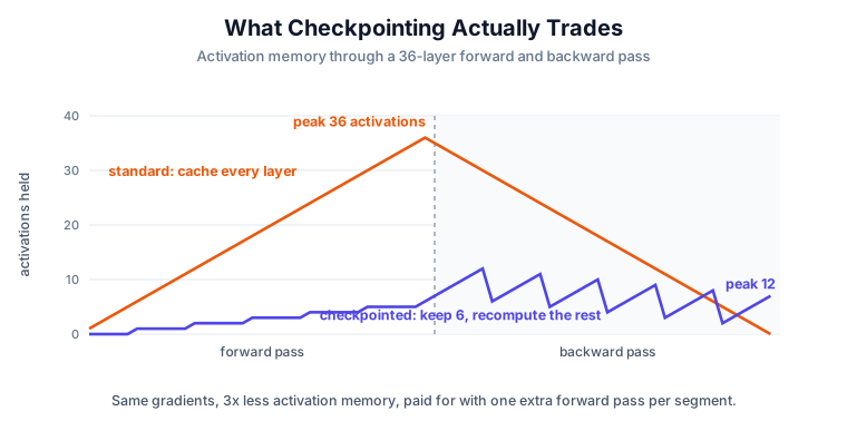
The standard curve is a triangle: memory climbs through the forward pass as every layer’s activations are cached, peaks at 36, then drains as backward consumes them. The checkpointed run holds only 6 checkpoints through the entire forward pass, then sawtooths during backward as it recomputes one segment at a time and releases it. Peak drops from 36 to 12, a 3x saving, and the sawtooth is literally the recomputation you are paying for.
The segment size is the knob. Keeping every \(\sqrt{n}\)-th activation balances the checkpoints you store against the buffer you need while recomputing, which is where the \(O(\sqrt{n})\) comes from.
model.gradient_checkpointing_enable()          # transformers
# or, per block:
from torch.utils.checkpoint import checkpoint
h = checkpoint(block, h, use_reentrant=False)  # use_reentrant=False is the modern path
Trap: “if it recomputes dropout, does it get different masks?” It would, and that would silently corrupt your gradients. PyTorch preserves and restores the RNG state across the recompute so the second forward pass is identical. Knowing that the question has an answer, rather than assuming it is broken or assuming it is magic, is the signal.
Where the memory actually goes, and which tool attacks which part:
| Memory consumer | Roughly | Attacked by |
|---|---|---|
| Parameters | \(P\) | FSDP/ZeRO sharding, quantization |
| Gradients | \(P\) | FSDP/ZeRO, LoRA (only adapters get gradients) |
| Optimizer state | \(2P\) for Adam | 8-bit Adam, Lion/Muon, ZeRO stage 1 |
| Activations | batch x sequence x layers | Gradient checkpointing, smaller micro-batch |
That table is the answer to “the model does not fit, what do you do?” Name the four consumers, then name the tool that targets the one that is actually binding. Reaching for checkpointing when your problem is optimizer state, or for 8-bit Adam when your problem is a 32k-token sequence, is the wrong move at the right vocabulary.
7.4 Optimizer Memory
Adam keeps two extra tensors the size of your model. This is not an academic detail; it is often the binding constraint on what you can train.
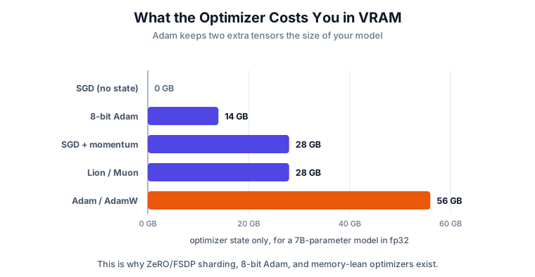
Those bars are optimizer state only, on top of the parameters, the gradients, and every activation you are holding for the backward pass. Switching from Adam to a single-state optimizer frees 28 GB on a 7B model, which can be the difference between fitting on your GPUs and not. This is a real engineering tradeoff, not a footnote.
For a 7B model in fp32, Adam’s \(m\) and \(v\) alone are about 56 GB, before parameters, gradients, or activations. This is why the ecosystem exists: ZeRO / FSDP shard optimizer state across GPUs, 8-bit Adam quantizes the states, and memory-lean optimizers like Lion and Muon are attractive at scale for exactly this reason.
7.5 Mixed Precision
Train in fp16 or bf16 for speed and memory, keep an fp32 master copy of the weights for the update. With fp16 you also need loss scaling, multiplying the loss by a large constant so small gradients do not underflow to zero in fp16, then unscaling before the step. bf16 has the dynamic range to skip this, which is a large part of why it is now preferred.
8. When the Loss Will Not Go Down
The diagnostic table. This is what a practical interview question actually looks like.
| Symptom | Most likely cause | What to try |
|---|---|---|
Loss is nan | LR too high, fp16 overflow, log(0) | Lower LR, add clipping, check for log of zero |
| Loss flat from step 0 | LR far too low, or no gradient reaching the params | Print gradient norms, check requires_grad |
| Loss drops then explodes | LR too high for the later landscape | Add warmup, add decay, clip |
| Loss bounces, no trend | LR too high or batch too small | Lower LR, accumulate gradients |
| Train falls, val rises | Overfitting | Regularize, augment, stop earlier |
| Both plateau high | Underfitting, or a dead architecture | Bigger model, check for dead units, raise LR |
| Fine alone, broken multi-GPU | Gradients not syncing, or effective LR changed | Check the scaling rule and reduction |
The first move is always the same: print the gradient norm. A norm of zero means nothing is reaching your parameters and the optimizer is irrelevant. A norm of \(10^{6}\) means you need clipping. A norm that looks sane means the problem is elsewhere, and you have eliminated half the search space in one line.
9. Rapid-Fire Q&A
SGD or Adam? Adam (AdamW) converges faster with far less tuning and is the default. Well-tuned SGD with momentum still matches or beats it on some vision benchmarks and generalizes slightly better. For transformers it is not a real contest: AdamW.
Why is Adam faster to converge but sometimes worse at generalizing? The per-parameter scaling lets it race down the loss surface, but it tends to land in sharper minima than SGD’s noisier path. AdamW’s decoupled decay closed most of the practical gap.
What does \(\epsilon\) do in Adam? Prevents division by zero, and quietly caps the maximum step size. Raising it (say \(10^{-6}\)) is a real stabilization trick for training that keeps blowing up.
Momentum \(\beta = 0.9\) means what? Roughly an average over the last ten gradients, since \(1/(1-\beta) = 10\).
Why warmup specifically for Adam? Its second-moment estimate is built from almost no data in the early steps, so the adaptive denominator is unreliable exactly when a bad step is most costly.
Can the learning rate be too small? Yes, and it is worse than it sounds. You do not just train slowly; you can settle into a poor region because you never had enough step size to escape it, and you burn your compute budget finding out.
Second-order methods: why not? Newton’s method needs the Hessian, which is \(N \times N\) for \(N\) parameters. At a billion parameters that matrix does not fit in any universe. Every practical second-order method (Sophia, Shampoo) is an approximation that avoids ever forming it.
What actually changes between finetuning and pretraining? Much lower learning rate (often 10x to 100x), shorter or no warmup, and a linear rather than cosine decay. The model starts in a good region and you are trying not to destroy it.
Adam with batch size 1? It works, but the second-moment estimate becomes very noisy, so you are adapting per-parameter step sizes from almost no signal. Accumulate gradients instead.
Accumulation or checkpointing? Different problems, and they compose. Accumulation buys you a large effective batch on small hardware; checkpointing buys you a larger micro-batch or a longer sequence for the same memory. Out of memory, reach for checkpointing. Batch too small to train stably, reach for accumulation. Most large runs use both, plus sharding.
Why is the loss identical for a few steps then diverges under accumulation? Almost always the missing loss division, or clipping applied inside the accumulation loop instead of before the step. Both are invisible until the gradient gets large enough to matter.
The Idea Underneath
Every optimizer in this post is answering one question: given a noisy estimate of which way is downhill, how much should you trust it?
SGD trusts each gradient completely and takes a fixed step. Momentum trusts the recent trend more than any single gradient. Adam trusts each parameter’s direction in proportion to how consistent its history has been. Muon trusts the momentum matrix’s direction but refuses to let a few dominant directions absorb the whole update.
The loss says what you want. The architecture says what you can represent. The optimizer decides how much to believe each noisy step you take toward it, and the learning rate is you telling it how brave to be.