Part of a series with loss functions, activation functions, optimization and metrics. Those cover how a model trains and how you judge it. This one is about picking the right model in the first place, and knowing what it is actually doing.
If you can’t say which model fits a problem and roughly what it does internally, the title on your badge is doing a lot of work. So let’s fix that.
1. Pick in 60 Seconds
| Your data | Start here | Then try | Skip |
|---|---|---|---|
| Tabular, typical / large | logistic / linear regression | gradient boosting (XGBoost, LightGBM, CatBoost) | a net as the first move |
| Tabular, small (<~50k rows) | logistic / linear | TabPFN, then GBDT | training a net from scratch |
| Tabular, must explain it | logistic / linear (Ridge) | GAM / EBM, then GBDT + SHAP | anything deep |
| Images | fine-tune a pretrained CNN or ViT | train from scratch if you truly have the data | classical CV features |
| Text classification | TF-IDF + logistic (as a baseline) | fine-tune a small encoder | RNN, LSTM |
| Time series, business data | seasonal naive, then GBDT on lags | a time-series foundation model if you have many related series | LSTM as the first move |
| No labels, want groups | k-means | HDBSCAN when clusters are messy | forcing supervision |
| No labels, find outliers | Isolation Forest | density / reconstruction | k-means as an anomaly detector |
| Find similar things | embeddings + ANN search | learned retrieval | exact kNN at scale |
| Barely any labels | pretrained model + fine-tune | semi-supervised, active learning | training from scratch |
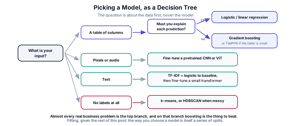
The honest summary: almost every real business problem is a table. On a table you still start with a linear baseline and then GBDT. On a small table, a tabular foundation model (TabPFN) is now a real alternative to tuning boosting. Everything else on this list is a specialization.
2. Always Start With a Baseline
Before any modeling, build the dumbest thing that produces a number: predict the majority class, predict the mean, or run logistic regression on your five most obvious features.
This takes twenty minutes and buys you two things you cannot get any other way. It tells you whether the problem is even hard (if logistic regression hits 0.94 AUC, your fancy model is fighting for scraps), and it gives you a floor that makes every later result interpretable. “XGBoost got 0.91” means nothing on its own. “XGBoost got 0.91, logistic got 0.89” means something very specific: you spent two weeks for two points.
Interview tell: candidates who jump straight to “I’d use a neural network” without asking about data size, feature types, or latency have usually not shipped anything. The first question is always about the data, never about the model.
The tabular reality
Deep learning transformed vision, audio and language. It has mostly not displaced gradient boosting on ordinary tabular data, and that surprises people who learned ML from headlines.
The reasons are structural, not a matter of tuning harder:
- Tabular features are not interchangeable. Column 3 is “age” and column 7 is “zip code.” A dense net freely mixes columns unless you add the right structure; trees split on one column at a time, which matches how tabular rules are often written.
- Real tabular targets are jagged. Risk jumps at age 25 because of an insurance rule, not along a smooth curve. Trees model sharp thresholds natively; smooth networks have to work to approximate a step.
- Irrelevant columns are everywhere. Trees just never split on them. A dense layer has to learn to zero them out.
- Low preprocessing tax. No scaling, strong missing-value handling in modern GBDT libraries, and categorical support is practical in CatBoost, LightGBM, and recent XGBoost. You still need to encode the problem correctly, but you spend less time making the data numerically acceptable.
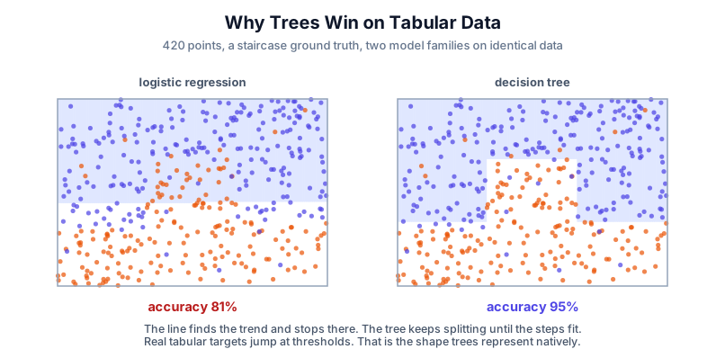
I generated 420 points where the true rule is a staircase, fit both, and measured. Logistic regression gets 81% and a decision tree gets 95% on identical data. The line finds the overall trend and then has nowhere left to go. The tree keeps splitting until the corners fit.
So the default serious model you train yourself on a table is still boosting. Trees still beat from-scratch nets on typical tabular data, for the four reasons above, and that has not flipped.
The 2025–2026 caveat is tabular foundation models. TabPFN is a transformer pretrained on millions of synthetic tables. You do not train it on your data: you feed labeled rows as context and it predicts in one forward pass. On small and medium tables it often matches a tuned GBDT with zero tuning. It wants a GPU, it is not a drop-in for a 50-million-row production ranker, and you still need GBDT when you care about CPU latency, monotonic constraints, or retraining on a laptop. Interview answer: small table, try TabPFN; large production table, still LightGBM or XGBoost.
Reach for a net you train yourself on tabular only when a net is uniquely good at the job: huge data, representation sharing across tasks, high-cardinality embeddings, or mixed inputs where the table is only one part of the model. AutoGluon is the “I have compute and I want the last points” button; it is an ensemble, not a model choice.
3. The Classical Models, and What They’re Doing
Each of these gets the same treatment: what it actually does, when to reach for it, where it breaks.
3.1 Linear and Logistic Regression
Inside: multiply each feature by a weight, add them up, add a bias. For binary classification, squash that sum through a sigmoid to get a probability; for multiclass, use softmax. Training just searches for the weights that minimize your loss.
$$\hat y = w_1x_1 + w_2x_2 + \dots + b \qquad p = \sigma(\hat y)$$Reach for it when: you need a baseline, you need to explain a decision to a regulator or a PM, you need calibrated probabilities, you need to extrapolate, or you have far more features than rows (text with TF-IDF is the classic case, and it is still shockingly competitive).
The production version is usually Ridge / Lasso / Elastic Net, not vanilla least squares. L2 (Ridge) is the default when features are collinear; L1 (Lasso) when you want a sparse subset; Elastic Net when you want a bit of both. Same model family, the regularizer is the difference between a baseline that works and one that explodes.
It breaks when: the relationship is non-linear or features interact. Linear models cannot learn “risky only if young and new customer” unless you hand-build that interaction. They also want scaled inputs.
The coefficient is the whole selling point: “each extra year of age multiplies the odds by 1.03” is a sentence a human can act on. SHAP on a boosting model is a local explanation of one prediction; a coefficient is a global statement about the world. Interviewers treat those as different things, because they are.
3.2 Decision Trees
Inside: look at every feature and every possible split point, pick the one that best separates the target, split the data in two, and recurse. “Best” means largest drop in impurity (Gini or entropy for classification, variance for regression). What you end up with is a flowchart of if-statements.
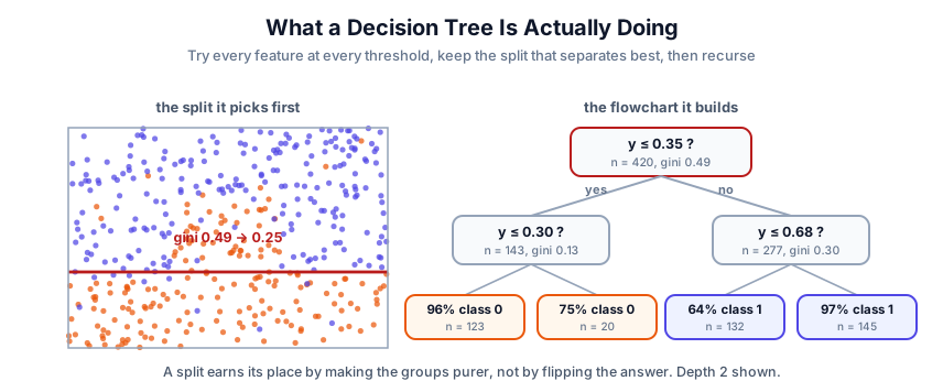
Look at the leaves on the right. The two on the left both predict class 0, which seems pointless until you read the percentages: 96% pure and 75% pure. A split earns its place by making the groups purer, not by flipping the answer. That is literally what the algorithm optimizes, and it is why trees keep splitting long after the prediction has stopped changing.
Reach for it when: you want something a non-technical stakeholder can literally read, or you need a fast, scale-free model on mixed data types.
It breaks when: you let it grow. A deep tree memorizes the training set perfectly and generalizes terribly. Trees are also unstable: change a handful of rows and you can get a completely different tree, because one different split at the top cascades.
That instability sounds like a fatal flaw. It is actually the opening for the next two models.
3.3 Random Forest: Average Away the Variance
Inside: train hundreds of trees, each on a bootstrap sample of the rows, and at each split let each tree consider only a random subset of features. Then average their predictions.
Both sources of randomness matter. Bootstrapping decorrelates the trees; restricting features stops every tree from locking onto the same one dominant predictor. Individually each tree is mediocre and overfit. Averaging many noisy-but-unbiased predictors cancels the noise.
Reach for it when: you want a strong result with almost no tuning. Random forests are remarkably hard to break and train in parallel. They also give feature importances quickly, though impurity-based importance is biased toward high-cardinality features; use permutation importance or SHAP when the explanation matters.
It breaks when: you need the last few points of accuracy (boosting usually wins), or you need to predict outside the training range. No tree model extrapolates. Train on houses up to 3,000 sq ft and ask about 5,000, and you get the answer for 3,000. Linear regression would happily extend the line. This is a favorite interview question and a real production failure.
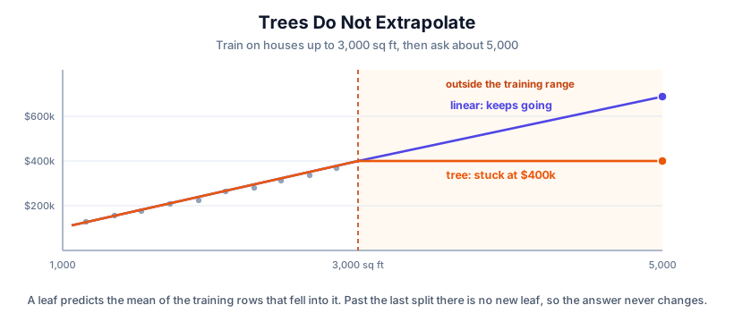
A leaf predicts the mean of the training rows that landed in it. Past the last split there is no new leaf, so the answer never changes. If your product actually needs “what happens at values we have not seen,” use a linear term, or an explicit trend feature, or don’t use a tree.
3.4 Gradient Boosting: The Tabular Champion
Inside: build trees sequentially, where each new tree is trained to predict the errors the ensemble has made so far. More precisely it fits the negative gradient of the loss, which for squared error is exactly the residual. Add each new tree’s output, scaled by a learning rate, to the running prediction.
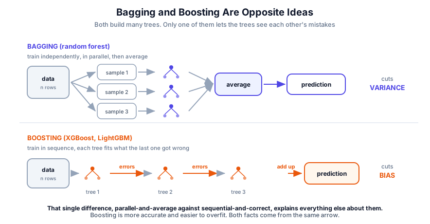
The difference from a forest is the whole idea. A forest builds trees in parallel and independently, then averages: that reduces variance. Boosting builds trees in sequence, each correcting the last: that reduces bias. Which is why boosting is more accurate and also easier to overfit.
The three implementations you will meet:
| Library | What it’s good at | The catch |
|---|---|---|
| XGBoost | The robust default, heavily battle-tested | Level-wise growth, a bit slower |
| LightGBM | Fastest on large data, leaf-wise growth | Leaf-wise overfits small datasets; cap num_leaves |
| CatBoost | Native categoricals, ordered boosting | Slower to train, fewer knobs |
sklearn HistGradientBoosting | Good enough, no extra dependency | Not the Kaggle winner |
The hyperparameters that actually matter, in order: learning_rate and n_estimators (they trade directly, so lower the rate and add trees), max_depth or num_leaves, then the regularizers min_child_weight, subsample, colsample_bytree. Always use early stopping on a validation set; it tunes n_estimators for you. You do not scale features for trees.
Three production facts that interviews probe:
- Boosting ranks well and is poorly calibrated. If the number is a pCTR, a risk score, or anything multiplied by a dollar value, run Platt scaling or isotonic regression on held-out data. Logistic is often better calibrated out of the box; that is one reason it still ships. (Metrics post.)
- Pass categoricals natively in CatBoost, and in recent XGBoost/LightGBM. One-hot encoding a zip code is how you make boosting slow and overfit. Target encoding (replace a category with the mean of the label) leaks if you compute it on the whole dataset; compute it on the training fold only, or use CatBoost’s ordered encoding.
- Monotonic constraints (“more income must not lower the score”) are a one-liner in GBDT libraries and a project in a net. Credit and pricing ask for this.
It breaks when: you skip validation-based tuning, you need calibrated probabilities and forget to fix them, or you retrain constantly under tight latency, since the sequential build is slower than a parallel forest. Modern defaults are decent; early stopping is what keeps them honest.
3.5 kNN, Which Is Now Vector Search
Inside: there is no training. Store the data. At prediction time, find the \(k\) closest points by distance and let them vote, or average them.
People file kNN under “simple thing from the textbook.” That is a mistake, because with embeddings attached it became one of the most important systems in modern ML. Encode your items as vectors, and “find the nearest neighbors” is semantic search, is recommendation candidate generation, is image search, is dedup.
The catch is that exact kNN scans everything, which is \(O(N)\) per query and hopeless at a billion vectors. So production uses approximate nearest neighbor: HNSW builds a navigable graph you can greedily walk, and libraries like FAISS and ScaNN make it fast. You trade a sliver of recall for orders of magnitude of speed.
Reach for it when: similarity is the task, or you need a candidate set to rank later.
It breaks when: the embedding is bad (the algorithm cannot fix a space where the wrong things are close), or dimensionality is high and everything becomes roughly equidistant.
3.6 K-Means and Clustering
Inside: pick \(k\) centroids, assign every point to its nearest one, move each centroid to the mean of its members, repeat until nothing moves. Use k-means++ for initialization; random init gets stuck.
Reach for it when: you want rough segments for exploration, or you need to compress a space into a few prototypes.
It breaks when: clusters are not roughly spherical and similar in size, which is most real data, or when you cannot justify \(k\). The elbow method is more of a vibe than a criterion; silhouette score is better. When clusters are irregular or there’s genuine noise, HDBSCAN is the better tool because it finds the number of clusters itself and is allowed to label points as noise instead of forcing everything into a group.
Say this out loud in an interview: clustering has no ground truth, so “it worked” means a human looked at the clusters and they meant something. Treat it as exploration, not as a result.
3.7 Nearby, and When You Actually Pick Them
Not the default, but two of these are real production tools:
- SVM finds the boundary with the widest margin, and the kernel trick lets it draw curved boundaries cheaply by computing similarities without ever building the high-dimensional space. Elegant, and it dominated the 2000s. It scales badly past ~100k rows and boosting beats it on the problems it used to own.
- Naive Bayes assumes every feature is independent given the class, which is obviously false and works anyway. Genuinely useful as a text baseline you can train in one second.
- Isolation Forest isolates outliers in fewer random splits than normal points. The unsupervised default for “is this row weird,” used in fraud, infra, and manufacturing. It is not a rare-class classifier; if you have labels, that is a different problem.
- GAM / EBM (explainable boosting): an additive of one shape-function per feature. Like linear regression, except each “coefficient” is a curve you can plot. Used when legal or risk needs more accuracy than logistic and still a picture per feature.
- HMM and LDA are names you should recognize. Sequence modeling went to transformers, topic modeling went to embeddings plus clustering.
4. When Deep Learning Is Actually the Answer
Here is the rule that survives contact with reality:
Reach for deep learning when your input is raw, high-dimensional, and structured: pixels, waveforms, text, graphs. Those are the cases where the features cannot be hand-written, so a model that learns its own features wins. When your input is already a table of meaningful columns, humans already did the feature engineering, and trees use that better.
4.1 The Plain Neural Net
Stacked layers of “multiply by a weight matrix, add a bias, apply a nonlinearity.” The nonlinearity is the whole point; without it, any stack of layers collapses into a single linear one (the activation post has the one-line proof). Training is backprop plus an optimizer, which is the optimization post.
On tabular data an MLP is usually a slower, fussier GBDT. Its real job is to be a component of something bigger.
4.2 CNNs: How a Model Sees
Inside: instead of connecting every pixel to every neuron, slide a small learned filter across the image and record how strongly it responds at each position.
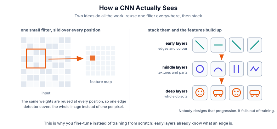
Two consequences do all the work. Weight sharing: the same edge detector is reused at every position, so you learn one filter instead of one per location, cutting parameters enormously and letting the model recognize a feature wherever it appears. Hierarchy: stack these and the first layers learn edges and colors, the middle layers learn textures and parts like wheels and eyes, and the deep layers learn whole objects. Nobody designed that progression; it falls out of training.
Weight sharing is also why a CNN is translation-equivariant: shift the cat, the detection shifts. Pooling then buys some invariance. That pair is the answer to “why not a big dense net on pixels.”
In practice you will almost never train one from scratch. You take a backbone pretrained on a large dataset (ResNet, ConvNeXt, ViT, DINOv2) and fine-tune it on your few thousand images, usually at a lower learning rate, sometimes freezing the early layers first. The early layers already know what an edge is, and edges are the same in every domain. Data augmentation (flip, crop, color jitter) is worth more than swapping one backbone for another. This is why “we only have 2,000 labeled images” is usually not fatal.
CNN vs ViT in one line: CNN is still the right default on small image sets; ViT pulls ahead when you have data, compute, and a strong pretrain. For an interview, the architecture brand name matters less than “pretrained, then fine-tune.”
4.3 Sequences, and Why RNNs Lost
RNNs and LSTMs process a sequence one step at a time, carrying a hidden state. LSTMs added gates so the state could hold information for longer. They were the standard for years.
They lost for a reason that has nothing to do with accuracy: they cannot be parallelized across time. Step 50 needs step 49 finished. When transformers arrived and could process an entire sequence at once on a GPU, the scaling argument ended the debate.
Do not reach for an LSTM on new work unless you have a specific constraint that makes recurrence useful. What replaced it, and how attention actually functions, is the next post.
And a note that saves real time: for time series forecasting on business data, start even dumber than GBDT. A seasonal naive (“this week equals last year”) is the baseline that embarrasses a surprising number of sequence models. Then gradient boosting on lag features, rolling means, and calendar flags. Chronos / TimesFM-style foundation models are a reasonable next try when you have many related series. Do not reach for an LSTM first.
5. What Decides Projects More Than Model Choice
You will lose more accuracy to these than to picking the second-best algorithm.
Leakage is the number one killer, and it always looks like great results. Your model sees something at training time it will not have at prediction time. Classic forms: a column computed after the outcome (account_closed_date predicting churn), a random split on temporal data so the model trains on the future, rows from the same user split across train and test, or target encoding computed on the whole dataset. If your AUC is suspiciously high, look for leakage before you celebrate.
Your validation split must match how the model will be used. Time-dependent problem means a time-based split. Grouped data (multiple rows per customer) means a group split. A random split on either quietly inflates every number you report.
Imbalance is usually a threshold and metric problem, not a modeling one. Move the threshold, use class weights, and measure with PR-AUC (see the metrics post). Reach for resampling after those, not before, and be skeptical of SMOTE on high-dimensional data.
Features still matter on tabular data. Ratios, differences, aggregates over time windows, count encodings. A good feature beats a better model regularly, and unlike the model it usually transfers to the next problem.
Drift means the world moved after you shipped. Monitor input distributions and the live metric, and decide your retraining cadence up front rather than after the incident.
6. What It Costs to Run
Accuracy you cannot serve is not accuracy.
| Model | Train | Predict | Size | Typical use |
|---|---|---|---|---|
| Logistic / Ridge | seconds | microseconds | KB | High-QPS, interpretable |
| Random forest | minutes, parallel | fast | 10s of MB | Solid default |
| Gradient boosting | minutes to hours | fast, CPU | MB | The tabular default you ship |
| TabPFN | none (pretrained) | GPU, ms–s | the foundation model | Small/medium tables |
| Isolation Forest | seconds to minutes | fast | small | Unsupervised outliers |
| kNN / ANN | none, plus index build | depends on index | large (all vectors) | Retrieval |
| Fine-tuned CNN | hours on GPU | ms on GPU | 10s to 100s of MB | Vision |
The questions that decide the architecture: what’s the latency budget, how often does this retrain, does it need a GPU at inference, and can you explain a single prediction when someone asks. A 0.5% AUC gain that doubles p99 latency is usually a losing trade, and knowing that is the difference between an ML engineer and someone who has read about ML.
7. Rapid-Fire Q&A
Default model for a new tabular problem? Logistic or linear regression as the baseline, then LightGBM or XGBoost with early stopping. On a small table, add TabPFN to that bake-off. That covers most of what you will ever be handed.
TabPFN or XGBoost? TabPFN when the table is small or medium and you want a strong answer with no tuning. XGBoost/LightGBM when the table is large, you need CPU inference, monotonic constraints, or a model you retrain in production every day.
Random forest or gradient boosting? Forest when you want a strong answer with no tuning and no overfitting worry. Boosting when you want maximum accuracy and will actually tune. Boosting usually wins by a few points.
Why do trees beat neural nets on tabular data? Tabular features are individually meaningful and targets are jagged. Trees split per-column and model sharp thresholds natively; nets are rotation-invariant and biased toward smooth functions, which is the wrong prior here. From-scratch nets still lose on ordinary tables. TabPFN is a different move: it is a pretrained prior, not a net you train on the table.
Bagging vs boosting in one line? Bagging trains independently in parallel and averages to cut variance. Boosting trains sequentially on the previous errors to cut bias.
Can a random forest overfit? Barely, by adding trees. It overfits through very deep individual trees and through leakage. Boosting overfits easily, which is why early stopping is not optional.
Why won’t my tree model extrapolate? A tree predicts the mean of a training leaf. Outside the training range there is no leaf, so it returns the boundary value forever. Use a linear model or an explicit trend term when extrapolation matters.
When would you actually pick linear regression over boosting? When you must explain coefficients, when data is tiny, when you need extrapolation, when you need calibrated probabilities without a second stage, or when p is much larger than n.
Does boosting give you probabilities you can trust? Not out of the box. Calibrate. Logistic often needs no such fix.
How do you choose k in k-means? Silhouette score over the elbow method, checked against whether the clusters mean anything to a human. If the answer is genuinely unclear, HDBSCAN removes the question.
Unsupervised anomaly detection? Isolation Forest first. k-means is a clustering tool that people misuse as an anomaly detector.
Is kNN obsolete? The opposite. With embeddings and an ANN index it is the retrieval layer under semantic search and RAG.
Only 500 labeled examples? Pretrained model plus fine-tuning, simple models with heavy regularization, cross-validation instead of a single holdout, and a serious look at whether you can get more labels.
The Idea Underneath
Every model here is a different bet about what shape the answer has.
Linear regression bets it’s a straight line. Trees bet it’s a stack of thresholds. kNN bets similar inputs give similar outputs. CNNs bet that meaning is local and repeats across position. TabPFN bets that a prior over synthetic tables is a better starting point than learning one table from scratch. Each is a strong assumption, and each wins exactly when its assumption matches your data.
That’s why “which model” is really “what do I believe about this problem,” and why the answer starts with looking at the data instead of the leaderboard. Interviewers ask about models because the answer reveals whether you’ve ever actually looked.