The companion to Every Loss Function You Need to Ace Your ML Interview. The loss defines what “good” means; the activation decides what the network can express at all.
1. The 60-Second Table
| Activation | Formula | Range | Use it for | PyTorch |
|---|---|---|---|---|
| ReLU | \(\max(0,x)\) | \([0,\infty)\) | The default for CNNs and MLPs | nn.ReLU |
| Leaky ReLU | \(\max(\alpha x, x)\) | \((-\infty,\infty)\) | When units are dying | nn.LeakyReLU |
| PReLU | learnable \(\alpha\) | \((-\infty,\infty)\) | When you can afford the params | nn.PReLU |
| ELU | \(x\) or \(\alpha(e^x-1)\) | \((-\alpha,\infty)\) | Smooth, negative-capable | nn.ELU |
| GELU | \(x\,\Phi(x)\) | \(\approx(-0.17,\infty)\) | Transformers (BERT, GPT) | nn.GELU |
| SiLU / Swish | \(x\,\sigma(x)\) | \(\approx(-0.28,\infty)\) | Deep nets, EfficientNet | nn.SiLU |
| SwiGLU | gated Swish | unbounded | Modern LLM feedforward blocks | custom |
| Tanh | \(\tanh(x)\) | \((-1,1)\) | RNN/LSTM gates, zero-centered need | nn.Tanh |
| Sigmoid | \(1/(1+e^{-x})\) | \((0,1)\) | Output for binary/multilabel | nn.Sigmoid |
| Softmax | \(e^{z_k}/\sum_j e^{z_j}\) | \((0,1)\), sums to 1 | Output for multiclass | nn.Softmax |
The short version: ReLU in hidden layers unless you have a reason; GELU or SwiGLU in transformers; sigmoid and softmax only at the output; tanh when you specifically need a zero-centered bounded signal.
2. Why Any Activation At All
This is the warm-up question, and the answer is one line of algebra. Stack two linear layers with no nonlinearity between them:
$$W_2(W_1x+b_1)+b_2 = (W_2W_1)x + (W_2b_1+b_2)$$The result is a single affine map. A hundred stacked linear layers have exactly the representational power of one. Depth buys you nothing without a nonlinearity, which is the entire reason activations exist.
What makes a good one:
- Nonlinear, or depth collapses as above
- Differentiable (almost everywhere is enough) so gradients flow
- Cheap, since it runs on every unit on every forward and backward pass
- Well-behaved gradients, meaning it doesn’t systematically shrink or explode the signal across layers
That last property is where most of them fail, and it’s what the next two sections are about.
3. The Saturating Classics
3.1 Sigmoid
$$\sigma(x)=\frac{1}{1+e^{-x}}, \qquad \sigma'(x)=\sigma(x)(1-\sigma(x))$$Squashes into \((0,1)\), which reads like a probability. That made it the default for years. It has three problems that ended it as a hidden-layer choice.
Vanishing gradients. The derivative peaks at \(\sigma'(0)=0.25\) and falls toward zero in both tails. Backprop multiplies these together, so across \(n\) layers the gradient is scaled by at most \(0.25^n\). Ten layers gives you a factor of roughly \(10^{-6}\) in the best case, and far worse once units saturate. Early layers stop learning.
Not zero-centered. Outputs are always positive, so for a downstream weight vector every gradient component shares the sign of the incoming gradient. Updates can only move all-positive or all-negative, forcing an inefficient zigzag toward the optimum.
Cost. An exp per unit is meaningfully slower than a comparison against zero.
Trap: “why did we stop using sigmoid in hidden layers?” Lead with the 0.25 number. Saying “vanishing gradients” is the memorized answer; saying “its derivative maxes at 0.25, so gradients shrink at least fourfold per layer” is the understood one.
3.2 Tanh
$$\tanh(x)=\frac{e^{x}-e^{-x}}{e^{x}+e^{-x}}, \qquad \tanh'(x)=1-\tanh^2(x)$$A rescaled sigmoid: \(\tanh(x)=2\sigma(2x)-1\). Range \((-1,1)\), and crucially it is zero-centered, which fixes sigmoid’s second problem. Its derivative peaks at 1 rather than 0.25, so it vanishes more slowly.
It still saturates in both tails, so it is still a poor deep hidden-layer choice. It survives where a bounded, zero-centered signal is the point: LSTM and GRU cell states, and anywhere you need an output in \((-1,1)\).
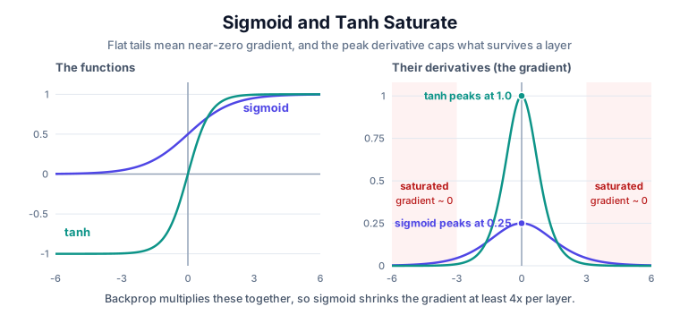
The right panel is the whole problem in one picture. Outside roughly \([-3,3]\) both derivatives are effectively zero, so a saturated unit passes almost nothing backward. And even at their best, in the very center, sigmoid tops out at 0.25 while tanh reaches 1.0. That ceiling is what compounds with depth.
4. The ReLU Family
4.1 ReLU
$$\text{ReLU}(x)=\max(0,x), \qquad \text{ReLU}'(x)=\begin{cases}1 & x>0\\ 0 & x\lt 0\end{cases}$$The change that made deep networks trainable. For positive inputs the gradient is exactly 1, so it neither shrinks nor grows as it propagates: no saturation, no vanishing. It is also a single comparison, so it’s essentially free, and it produces sparse activations since roughly half the units output zero.
Dying ReLU is the price. If a unit’s pre-activation is negative for every input in the data (typically after a large gradient step drives its bias strongly negative), its output is 0, so its gradient is 0, so it never updates again. It is permanently dead, not merely inactive.
Trap: the follow-up is always “how would you detect and fix it?” Detect by logging the fraction of zero activations per layer; a layer stuck near 100% zeros has dead units. Fix by lowering the learning rate, which is the usual root cause, or switching to Leaky ReLU or GELU. Proper initialization (He/Kaiming for ReLU) prevents most of it up front.
Trap: “ReLU isn’t differentiable at 0, so how does backprop work?” The kink is a single point, measure zero, and float inputs essentially never land exactly there. Frameworks just pick a subgradient; PyTorch defines the derivative at 0 as 0. It has never mattered in practice.
4.2 Leaky ReLU and PReLU
$$\text{LeakyReLU}(x)=\max(\alpha x, x), \quad \alpha \approx 0.01$$Give the negative side a small slope so the gradient is never exactly zero and dead units can recover. PReLU makes \(\alpha\) a learned parameter instead of a constant.
In practice the improvement over plain ReLU is real but modest, and inconsistent across tasks. It’s the first thing to try when you have measured a dying-unit problem, not a default.
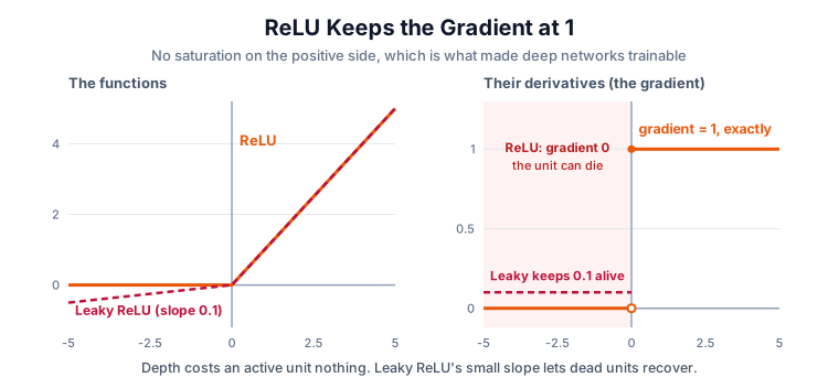
Compare that right panel with the previous one. There is no peak and no decay: for any active unit the gradient is exactly 1, so it passes through a layer unchanged no matter how deep the stack. The cost is the shaded region, where ReLU’s gradient is exactly zero and a unit that lands there can never come back. Leaky ReLU’s small negative slope is precisely the fix for that.
Stack the two behaviors across depth and the gap is not subtle:
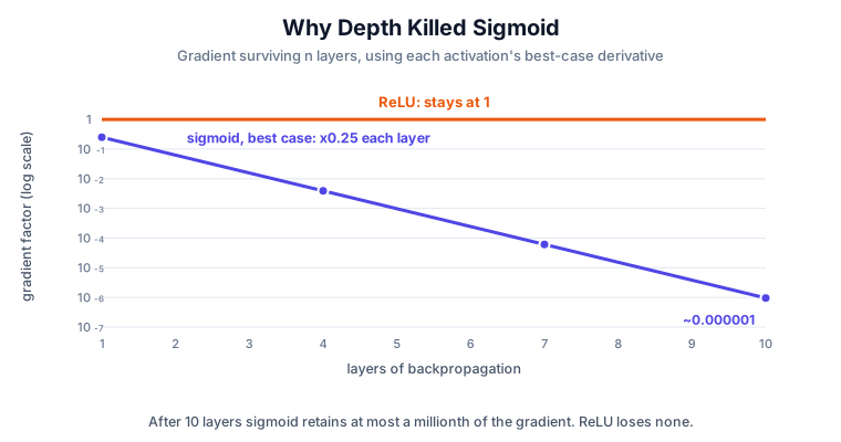
Both curves are best cases, which is what makes the comparison fair and the result stark. Sigmoid is generous here (real units saturate and do worse), yet it still gives up roughly six orders of magnitude over ten layers, while ReLU gives up nothing. This is the vanishing gradient problem, and it is the single biggest reason deep learning became practical.
4.3 ELU and SELU
$$\text{ELU}(x)=\begin{cases}x & x>0\\ \alpha(e^{x}-1) & x\leq 0\end{cases}$$Smooth everywhere, with negative outputs that push the mean activation toward zero, recovering some of the zero-centering benefit. Costs an exp on the negative branch.
SELU is ELU with two specific fixed constants chosen so that activations converge to zero mean and unit variance across layers, making the network self-normalizing. The catch is that the guarantee only holds with lecun_normal initialization, AlphaDropout, and a plain feedforward stack. Break any of those and it’s just a scaled ELU. That fine print is why it never displaced BatchNorm.
4.4 GELU
$$\text{GELU}(x)=x\,\Phi(x)$$where \(\Phi\) is the standard normal CDF. Instead of ReLU’s hard gate (keep or zero), GELU weights the input by the probability that a standard normal draw falls below it, so the gate is smooth and stochastic in spirit.
The common approximation, which is what most implementations ship:
$$0.5x\left(1+\tanh\left(\sqrt{2/\pi}\,(x+0.044715x^{3})\right)\right)$$It is smooth, non-monotonic near zero, and allows small negative outputs, so there are no dead units. This is the activation in BERT and the GPT family, and the default choice for transformer feedforward blocks.
4.5 SiLU / Swish
$$\text{SiLU}(x)=x\,\sigma(x)$$Found by architecture search and published as Swish. Shaped very much like GELU: smooth, non-monotonic, with a small negative dip around \(x\approx-1.28\). Cheaper than GELU’s exact form and used in EfficientNet and many LLM stacks.
Trap: “GELU vs SiLU, which is better?” They perform within noise of each other on most benchmarks, and the honest answer says so. The real differentiators are implementation cost and what the rest of your architecture already assumes. Pick one and stay consistent; a confident claim that one is universally superior is a weaker answer than acknowledging the tie.
4.6 Mish
$$\text{Mish}(x)=x\tanh(\text{softplus}(x))$$Same smooth non-monotonic family, slightly more expensive, occasionally better in vision. Worth recognizing, rarely worth reaching for.
5. Gated Activations: What LLMs Actually Use
Modern LLM feedforward blocks mostly don’t use a plain activation. They use a gated linear unit, where one projection produces the signal and a second produces a multiplicative gate:
$$\text{GLU}(x)=(xW)\otimes\sigma(xV)$$Swap the gate’s nonlinearity and you get the family:
| Variant | Gate | Used by |
|---|---|---|
| GLU | sigmoid | original formulation |
| GeGLU | GELU | T5 v1.1, PaLM |
| SwiGLU | Swish / SiLU | LLaMA, Mistral, most modern open LLMs |
Why gating helps: the multiplicative interaction lets the layer suppress or amplify features conditionally, which a pointwise function applied to a single projection cannot do. Empirically it’s worth a consistent perplexity improvement at equal parameter count.
Trap: the good follow-up is “doesn’t that add parameters?” Yes. A gated block needs three weight matrices where a standard feedforward needs two. Implementations compensate by shrinking the hidden dimension, typically to \(\tfrac{2}{3}\) of what it would otherwise be, so total parameters stay roughly fixed and the comparison against a standard block is fair. If you can name that \(\tfrac{2}{3}\) adjustment, you have clearly read the architecture rather than the summary.
6. Output Activations
Hidden-layer activations shape what the network can represent. Output activations shape what it can mean, and they are chosen by the task, not by taste.
| Task | Output activation | Paired loss |
|---|---|---|
| Binary classification | Sigmoid | BCE |
| Multiclass, one label | Softmax | Cross-entropy |
| Multilabel | Sigmoid per label | BCE per label |
| Regression | None (linear) | MSE / MAE / Huber |
| Bounded regression | Sigmoid or tanh, rescaled | MSE |
Trap: putting ReLU on a regression output. It silently makes negative predictions impossible. If the target can be negative, the model can never be right, and the loss curve looks plausible while it happens.
Softmax, Properly
$$p_k=\frac{e^{z_k}}{\sum_j e^{z_j}}$$Shift invariance is the property that matters in practice:
$$\text{softmax}(z) = \text{softmax}(z - c)$$for any constant \(c\). Every real implementation subtracts \(c=\max_j z_j\) before exponentiating, because \(e^{1000}\) overflows to inf while \(e^{0}\) does not. Same answer, no overflow.
Temperature \(T\) rescales the logits before the exponential:
$$p_k=\frac{e^{z_k/T}}{\sum_j e^{z_j/T}}$$\(T\lt 1\) sharpens toward one-hot, \(T>1\) flattens toward uniform. This is the knob behind sampling temperature in LLM generation and behind softening teacher outputs in distillation.
Trap: the one that connects back to loss functions. Softmax is an activation; cross-entropy is the loss. And in PyTorch you must not apply softmax before
nn.CrossEntropyLoss, because it applieslog_softmaxinternally. Feeding it probabilities applies softmax twice and quietly flattens your gradients.
7. Choosing One
The decision, in order:
- Output layer? Task decides it. Use the table above and stop thinking.
- Transformer? GELU, or SwiGLU if you’re building the feedforward block yourself.
- CNN or MLP? ReLU with He initialization. It is still the right default.
- Units dying? Measure the zero fraction first. Then Leaky ReLU or GELU.
- RNN or LSTM? Tanh and sigmoid, because the gating mechanism is defined in terms of bounded, zero-centered signals.
- Anything else? Start with ReLU and only move if you have a measurement that says to.
The honest summary is that activation choice is rarely what limits a model. Architecture, data, and optimization dominate. Knowing that, and saying it, is a stronger interview answer than an enthusiastic ranking of exotic activations.
8. Rapid-Fire Q&A
Why did ReLU beat sigmoid? Constant gradient of 1 on the positive side, so no vanishing across depth, plus it’s far cheaper. Sigmoid’s derivative maxes at 0.25.
Vanishing vs exploding gradients? Vanishing is repeated multiplication by factors below 1 until early layers stop learning; exploding is repeated multiplication by factors above 1 until updates diverge. Activations mostly cause the first; poor initialization and recurrence cause the second. Gradient clipping addresses exploding, not vanishing.
Dead ReLU vs vanishing gradient? Different failures. A dead unit has a gradient of exactly zero, permanently, for every input. Vanishing gradients are nonzero but shrink multiplicatively with depth. One is a stuck unit, the other is a scaling problem.
Why is zero-centering good? If all activations entering a layer are positive, every weight’s gradient in that layer shares one sign, so updates zigzag instead of moving diagonally toward the optimum.
Can I use different activations in different layers? Yes, and you already do: hidden layers versus the output. Mixing within the hidden stack is legal but rarely helps and complicates reasoning.
Does BatchNorm change the choice? It reduces the pressure a lot, since normalizing pre-activations keeps units in the useful range and largely prevents the saturation ReLU was invented to dodge. It makes networks far more forgiving about activation choice.
Why GELU in transformers instead of ReLU? Smoothness and small negative outputs, which suit the deep residual stacks and large learning rates transformers use, plus no dead units. The empirical gain is small but consistent, and it’s now the convention.
Is softmax an activation or a loss? An activation. Cross-entropy is the loss. “Softmax loss” is informal shorthand for the pair.
Why no activation on a regression output? Any bounded activation caps the achievable range. A linear output can express any real value, which is what regression requires.
What initialization goes with what? He/Kaiming for ReLU-family (accounts for half the outputs being zero), Xavier/Glorot for tanh and sigmoid. Mismatched initialization is a common cause of a network that won’t train at all.
The Idea Underneath
Every activation here is trading off the same three things: how much gradient survives backprop, how much it costs to compute, and how much it can express.
Sigmoid maximized interpretability and lost the gradient. ReLU maximized gradient flow and lost the negative half. GELU and SwiGLU bought some of that back with smoothness and gating, paying in FLOPs.
There is no best activation, only the one whose trade-off matches your depth, your architecture, and your compute budget. If you’re unsure, ReLU is still a defensible answer, and knowing why it’s defensible is the actual question being asked.